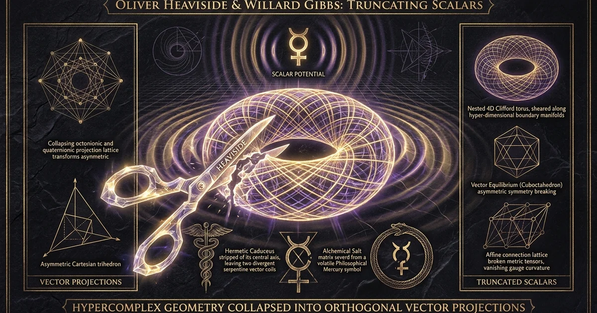
Oliver Heaviside and Willard Gibbs: Truncating Scalars

Executive Summary & Theoretical Thesis

The Geometrical Topology of Maxwell’s Original Hypercomplex Formulation

In his foundational 1865 memoir, A Dynamical Theory of the Electromagnetic Field, and his subsequent 1873 masterwork, A Treatise on Electricity and Magnetism, James Clerk Maxwell did not express electrodynamic laws via the four compact vector equations taught in contemporary physics. Instead, Maxwell formulated a comprehensive system of twenty coupled differential equations possessing twenty variable quantities. Central to this architecture was William Rowan Hamilton’s algebra of quaternions—a non-commutative, associative division ring over the real numbers denoted by $\mathbb{H}$. In Maxwell’s conception, the electromagnetic field was intrinsically hypercomplex. Hamilton’s biquaternions united three-dimensional spatial vectors with an invariant real scalar part, establishing an eight-dimensional algebraic field structure that coupled transverse spatial rotational mechanics with longitudinal, non-rotational energetic gradients.

By deploying Hamilton’s system, Maxwell possessed a mathematical language wherein field quantities were naturally unified rather than split into disparate computational components. The electromagnetic momentum—designated by Maxwell as the electrokinetic momentum vector $\mathbf{A}$—and the electrostatic scalar potential $\Phi$ did not operate as arbitrary mathematical artifices or mere gauge conveniences. Rather, they constituted the foundational primary reality of the field: a unified hypercomplex potential field possessing genuine physical ontology. Within this framework, field interactions inevitably yielded real scalar invariants representing localized energetic stress, volumetric pressure, and longitudinal vacuum displacement. Transverse electromagnetic radiation represented merely the rotational, divergence-free facet of a broader dynamical system governed by hypercomplex spatial topology.

This unified field ontology, detailed further in the analysis of quaternion Maxwell equations formulations, demonstrated that Maxwell’s early electrodynamics accommodated structural states fundamentally inaccessible to decoupled vector representations. The hypercomplex field mapped dynamics across an elastic, dielectric continuum wherein topological twists, localized phase boundaries, and scalar surges were mathematically coherent. By embedding both the rotational cross-product mechanics and the contractile scalar dot-product mechanics into a singular hypercomplex operator, Maxwell retained the geometric continuity between scalar stress fields and transverse electromagnetic waves.

The Heaviside-Gibbs Vector Reduction and the Excision of Scalar Realities

Between 1881 and 1893, self-taught English telegraph engineer Oliver Heaviside and American mathematical physicist Josiah Willard Gibbs initiated a radical reconstruction of electrodynamic theory. Observing that Hamilton’s quaternion system presented formidable computational friction to practicing engineers and physicists—principally due to the sign conventions and the irreducible integration of scalar and vector quantities—Heaviside and Gibbs deliberately excised the scalar real part of the quaternion. They severed Hamilton’s unified product into two distinct, disconnected mathematical operations: the scalar dot-product ($\mathbf{p} \cdot \mathbf{q}$) and the vector cross-product ($\mathbf{p} \times \mathbf{q}$).

pq = -p · q + p × q

This operational bifurcation catalyzed what is documented in historical physics as the heaviside gibbs vector truncation maxwell four equations. Heaviside condensed Maxwell’s twenty governing relations down to the canonical quartet of asymmetric vector differential equations utilizing the newly minted differential operators curl ($\nabla \times$) and divergence ($\nabla \cdot$). In carrying out this vector analysis simplification, the scalar potential was systematically demoted. Gibbs and Heaviside discarded the dynamic status of the scalar real term, treating it as an algebraic nuisance that lacked direct mechanical measurability via standard Galvanic deflection needles.

The immediate structural consequence was the total elimination of scalar potentials as primary physical agents. The electric field vector $\mathbf{E}$ and the magnetic field vector $\mathbf{B}$ were elevated to fundamental ontological status, while the vector potential $\mathbf{A}$ and the scalar potential $\Phi$ were relegated to secondary mathematical constructs—calculational stepping stones devoid of physical reality. This deliberate vectorization discarded the possibility of dynamical scalar field dynamics in free space, cementing an electrodynamic paradigm that recognized only transverse field oscillations operating at light velocity $c$.

Thermodynamic and Topological Consequences of Eliminating Scalar Dynamics

The structural truncation of the quaternion field to asymmetric vector pairs introduced profound thermodynamic and topological limitations into classical field theory. When the dynamic scalar components of the field were eliminated, electrodynamics lost the capacity to express non-equilibrium energy exchanges occurring between the transverse wave vectors and the underlying vacuum potential field. In a fully hypercomplex framework, the divergence of a vector potential field does not vanish automatically; instead, it couples directly to time-varying scalar potentials, generating longitudinal waves characterized by localized stress transitions and compressive density oscillations within the medium.

By forcing electrodynamics into a purely transverse paradigm, the Heaviside-Gibbs formulation necessitated arbitrary gauge fixing conditions—most notably the Coulomb gauge ($\nabla \cdot \mathbf{A} = 0$) and the Lorenz gauge ($\nabla \cdot \mathbf{A} + \frac{1}{c^2} \frac{\partial \Phi}{\partial t} = 0$). These gauge constraints served as mathematical duct-tape, implemented precisely to prevent the orphaned scalar degrees of freedom from destabilizing the truncated vector equations. Consequently, energy conservation laws were artificially constrained to Poynting vector flux configurations:

$$\mathbf{S} = \frac{1}{\mu_0} (\mathbf{E} \times \mathbf{B})$$

This formulation fundamentally ignores non-Poynting scalar energy densities that do not propagate as transverse spatial cross-products.

Topologically, this vector reduction flattened the dynamic vacuum from a hypercomplex, multi-layered dielectric matrix into an inert, passive void. The excision of the real scalar component made it mathematically impossible to model macroscopic vacuum polarizations, continuous topological soliton states, or acoustic-type longitudinal dielectric pulses without invoking elaborate non-linear boundary patches. The historical loss of quaternion depth severed classical physics from a direct mathematical trajectory toward unified field theories, generating persistent foundational anomalies that would resurface throughout twentieth-century quantum mechanics.

Historical Lineage & Experimental Precedents

Hamiltonian Quaternions versus Gibbsian Pragmatism

The development of hypercomplex mechanics began on October 16, 1843, along the Royal Canal in Dublin, when William Rowan Hamilton inscribed the fundamental formula of quaternion algebra into the stone of Brougham Bridge:

$$i^2 = j^2 = k^2 = ijk = -1$$

Hamilton’s vision extended far beyond linear algebra; he perceived the quaternion as an ontological bridge unifying time (the one-dimensional real scalar axis) and space (the three-dimensional imaginary vector axes). His Scottish disciple, Peter Guthrie Tait, fiercely advanced the philosophy that quaternions constituted the native language of physical dynamics. Tait argued that to split a quaternion was to commit geometric violence against the structural integrity of natural physical law.

       Quaternion Space H
   [ Scalar: t / Energy Density ]
                 +
   [ Vector: x, y, z / Rotation ]
                 │
                 │  Heaviside-Gibbs Truncation
                 ▼
          3-Vector Space R³
       [ Dot Product: p · q ]
       [ Cross Product: p × q ]

By contrast, Josiah Willard Gibbs, working within the pragmatic empirical milieu of Yale University in the early 1880s, viewed Hamilton’s overarching philosophy as an unnecessary metaphysical burden. Gibbs privately printed his pamphlet Elements of Vector Analysis between 1881 and 1884 to provide students and physical chemists with an intuitive, utilitarian tool. Gibbs recognized that for the vast majority of Cartesian laboratory calculations—calculating static mechanical equilibrium, fluid fluxes, and basic magnetic forces—the full non-commutative machinery of quaternions was unwieldy. By separating the dot and cross operations, Gibbs gave physics a frictionless computational calculus, but did so at the expense of abandoning the algebraic division-ring property that made Hamilton’s space complete.

The Transatlantic Cable Problem: Heaviside’s Telegrapher’s Equations

Concurrently, Oliver Heaviside confronted the severe, real-world electrical problems plaguing long-distance telegraphy and submarine transmission cables. The British Post Office, under the technical direction of William Preece, was locked in an engineering crisis characterized by extreme signal degradation and dispersion along transoceanic copper lines. Signals transmitted as crisp square pulses arrived at receiving terminals as smeared, illegible dynamic plateaus. Heaviside, an outsider working with exceptional mathematical intuition, set out to solve this transmission failure using Maxwell’s electrodynamic theory.

To render Maxwell’s twenty equations practically applicable to distributed transmission-line parameters, Heaviside developed the Telegrapher’s Equations, explicitly calculating the interplay of resistance ($R$), inductance ($L$), conductance ($G$), and capacitance ($C$):

$$\frac{\partial V}{\partial x} = -L \frac{\partial I}{\partial t} - R I, \quad \frac{\partial I}{\partial x} = -C \frac{\partial V}{\partial t} - G V$$

Through this formulation, Heaviside discovered the “distortionless condition” ($RC = LG$), demonstrating that deliberately adding inductive loading to lines could mitigate dispersion and permit clear, high-speed telegraphic communication over continental distances.

This monumental engineering triumph cemented Heaviside’s faith in operational calculus and functional vector analysis. For Heaviside, electrodynamics was an engineering science of tangible energy flows along conductors and through the surrounding insulating dielectric field. Quaternion algebra, with its complex spatial transformations and negative signs arising from square-root operations, appeared to him as a pedantic obstruction. Heaviside’s overriding objective was to eliminate any mathematical formalism that could not be mapped directly to current, voltage, transverse electric fields, and magnetic flux loops.

The Great Vector Debate: Tait, Heaviside, and the Marginalization of Hypercomplex Algebra

The historical period between 1890 and 1894 witnessed an intense scientific polemic across the pages of Nature and the Philosophical Magazine, known as “The Great Vector Debate.” Peter Guthrie Tait, defending the quaternionic canon, attacked Heaviside and Gibbs as mathematical “depreciators” who were degrading Maxwell’s profound hypercomplex vision into a fragmented and mathematically defective shorthand. Tait argued that vector analysis was a parasitic hybrid that borrowed the fruits of quaternionic thinking while discarding its dynamic foundations, warning that the vector analysis simplification severed the organic connection between physical rotational forces and scalar field invariants.

Heaviside responded with ferocious, caustic polemics. He championed pragmatic functionality over mathematical orthodoxy, famously retorting that Tait’s pure quaternions were “a disease” that had arrested the development of Maxwellian electrodynamics for two decades. Gibbs contributed measured, devastating mathematical critiques highlighting that quaternion products could not be easily generalized to $n$-dimensional spaces or simple linear matrix operations.

       The Great Vector Debate (1890–1894)
       
  Tait (Quaternion Camp)      Heaviside & Gibbs (Vector Camp)
  ─────────────────────      ───────────────────────────────
  • Non-commutative division  • Disconnected dot/cross products
  • Unified scalar invariants • Explicit 3D spatial operators
  • Holistic continuum field  • Immediate telegraphic calculus
  • Rejection of truncation   • Pragmatic engineering hegemony

The vector camp triumphed entirely. Pragmatism, computational ease, and the rapid expansion of practical electrical engineering departments at the dawn of the twentieth century favored the Heaviside-Gibbs formulation. The physics academy standardized on the four vector equations, leaving quaternions to fade into mathematical obscurity. As a result, the deep ontological reality of the scalar field and the unified potential structure was largely forgotten, buried beneath a triumphant century of transverse circuit engineering.

Mathematical Formalism & Physical Mechanics

Derivation of the Octonion and Quaternion Electrodynamic Operators

To rigorously comprehend what was mathematically discarded during the Gibbs-Heaviside reduction, one must reconstruct the complete hypercomplex differential operator acting upon the potential field. Within Hamiltonian quaternion space $\mathbb{H}$, an arbitrary physical operator is defined by a real scalar differential component combined with a three-dimensional spatial differential operator. Let the four-dimensional hypercomplex gradient operator $\mathcal{D}$ be expressed as:

$$\mathcal{D} = \frac{1}{c}\frac{\partial}{\partial t} + \nabla = \frac{1}{c}\frac{\partial}{\partial t} + \mathbf{i}\frac{\partial}{\partial x} + \mathbf{j}\frac{\partial}{\partial y} + \mathbf{k}\frac{\partial}{\partial z}$$

where the basis elements satisfy the strict non-commutative relations $\mathbf{i}^2 = \mathbf{j}^2 = \mathbf{k}^2 = \mathbf{i}\mathbf{j}\mathbf{k} = -1$.

Similarly, the unified electromagnetic potential quaternion $\mathbf{\Lambda}$ combines the real scalar potential $\Phi$ with the three-dimensional vector potential $\mathbf{A}$:

$$\mathbf{\Lambda} = \frac{\Phi}{c} + \mathbf{A} = \frac{\Phi}{c} + \mathbf{i}A_x + \mathbf{j}A_y + \mathbf{k}A_z$$

The total electrodynamic field derivative is obtained via the quaternionic multiplication of $\mathcal{D}^*$ (the quaternionic conjugate operator $\frac{1}{c}\partial_t - \nabla$) and $\mathbf{\Lambda}$. Expanding this non-commutative product reveals how the scalar and vector components interlock dynamically:

$$\mathcal{F} = \mathcal{D}^* \mathbf{\Lambda} = \left( \frac{1}{c}\frac{\partial}{\partial t} - \nabla \right) \left( \frac{\Phi}{c} + \mathbf{A} \right)$$

Carrying out the expansion using the fundamental identity $\nabla \mathbf{A} = -\nabla \cdot \mathbf{A} + \nabla \times \mathbf{A}$, the product splits into its exact real scalar part and imaginary vector part:

$$\mathcal{F} = \left[ \frac{1}{c^2}\frac{\partial \Phi}{\partial t} + \nabla \cdot \mathbf{A} \right] + \left[ \frac{1}{c}\frac{\partial \mathbf{A}}{\partial t} + \frac{1}{c}\nabla \Phi - \nabla \times \mathbf{A} \right]$$

In this hypercomplex derivation, the real scalar bracket:

$$S = \frac{1}{c^2}\frac{\partial \Phi}{\partial t} + \nabla \cdot \mathbf{A}$$

is not zero by definition; it is a dynamic scalar invariant that represents volumetric vacuum dilation, dielectric field stress, and longitudinal displacement. The imaginary vector bracket comprises the classical magnetic flux density $\mathbf{B} = \nabla \times \mathbf{A}$ and the negative of the electric field intensity:

$$\mathbf{E} = -\nabla \Phi - \frac{\partial \mathbf{A}}{\partial t}$$

When extending this formalism to Cayley-Dickson octonions $\mathbb{O}$ (an eight-dimensional non-associative division algebra), the field encompasses sixteen degrees of freedom, inherently linking electromagnetic phenomena with gravitational stress fields and higher-dimensional rotational holonomies.

The Truncation Mechanism: Projective Mapping from H to R3

The Heaviside-Gibbs truncation acts mathematically as a non-invertible, projective reduction mapping $\pi: \mathbb{H} \to \mathbb{R}^3$. This projective mechanism strips the hypercomplex manifold of its real scalar domain, enforcing an explicit structural filter:

        Projective Truncation Mapping
        
  Quaternion Space H (4D)  ─────────┐
    • Scalar: S(t, x, y, z)          │
    • Vector: V(t, x, y, z)          │  π: H ──> R³
                                     │  (Excision of S)
  Vector Calculus R³ (3D)  ◄────────┘
    • Force Field: E = -∇Φ - ∂A/∂t
    • Flux Density: B = ∇ × A
    • Gauge Fix: S = 0 (Forced)

To execute this reduction, Heaviside enforced the condition that the dynamic scalar surge invariant must identically vanish:

$$S = \frac{1}{c^2}\frac{\partial \Phi}{\partial t} + \nabla \cdot \mathbf{A} = 0$$

By declaring $S = 0$ as an inviolable constraint rather than a dynamic variable, the dynamic scalar equation was permanently excised from electrodynamics. The hypercomplex field derivative was collapsed into four localized differential relations operating exclusively in three-dimensional Euclidean space:

$$\nabla \cdot \mathbf{E} = \frac{\rho}{\varepsilon_0}$$

$$\nabla \cdot \mathbf{B} = 0$$

$$\nabla \times \mathbf{E} = -\frac{\partial \mathbf{B}}{\partial t}$$

$$\nabla \times \mathbf{B} = \mu_0 \mathbf{J} + \mu_0 \varepsilon_0 \frac{\partial \mathbf{E}}{\partial t}$$

Through this mathematical compression, the scalar potential $\Phi$ ceased to be an independent dynamic field; it was transformed into a passive spatial boundary solution determined entirely by instantaneous charge configurations via Poisson’s equation $\nabla^2 \Phi = -\rho/\varepsilon_0$.

The physical mechanics of longitudinal waves—which fundamentally require non-zero variations in the scalar potential divergence term $S$ over time—were systematically barred from existing in free space. The vector equations mathematically restricted electrodynamic radiation in the vacuum exclusively to transverse oscillations traversing at the constant velocity $c = 1/\sqrt{\mu_0 \varepsilon_0}$.

Gauge Invariance as a Compensatory Artifact for Lost Scalar Potentials

A critical theoretical consequence of the Heaviside-Gibbs vector truncation was the artificial creation of gauge freedom. Because the potentials $\mathbf{A}$ and $\Phi$ were stripped of their primary physical status and reduced to computational intermediates for calculating the “real” fields $\mathbf{E}$ and $\mathbf{B}$, mathematicians recognized that these potentials were not uniquely defined. One could arbitrarily modify the potentials via the transformation:

$$\mathbf{A} \to \mathbf{A}’ = \mathbf{A} + \nabla \lambda$$

$$\Phi \to \Phi’ = \Phi - \frac{\partial \lambda}{\partial t}$$

where $\lambda(\mathbf{r}, t)$ is any arbitrary scalar field function, without changing the resulting physical fields:

$$\mathbf{B} = \nabla \times \mathbf{A}’ = \nabla \times (\mathbf{A} + \nabla \lambda) = \nabla \times \mathbf{A}$$

$$\mathbf{E} = -\nabla \Phi’ - \frac{\partial \mathbf{A}'}{\partial t} = -\nabla \left( \Phi - \frac{\partial \lambda}{\partial t} \right) - \frac{\partial}{\partial t}(\mathbf{A} + \nabla \lambda) = -\nabla \Phi - \frac{\partial \mathbf{A}}{\partial t}$$

Standard twentieth-century field theory celebrated gauge-invariance as a profound, elegant principle of fundamental physics. However, when viewed through the historical prism of hypercomplex algebra, gauge invariance is recognized as a compensatory artifact: an unphysical mathematical redundancy introduced precisely because the scalar dynamic degrees of freedom were amputated.

In a complete quaternion formulation, any transformation of the scalar or vector potential alters the dynamic scalar invariant $S$ and reconfigures the localized energy-momentum tensor of the hypercomplex field. The arbitrary gauge transformation $\lambda$ was necessitated only because classical vector electrodynamics broke the unified division ring of $\mathbb{H}$, leaving empty algebraic degrees of freedom that modern theory had to neutralize through global and local gauge fixing protocols.

Empirical Evidence & Observational Anomalies

The Aharonov-Bohm Effect: Re-emergence of Physical Potentials

For more than six decades following the Gibbs-Heaviside truncation, the orthodoxy that the electromagnetic potentials $\mathbf{A}$ and $\Phi$ were physically meaningless computational tools remained unchallenged in mainstream classical physics. This paradigm suffered a foundational breakdown in 1959 with the publication of Yakir Aharonov and David Bohm’s seminal paper, Significance of Electromagnetic Potentials in the Quantum Theory. Aharonov and Bohm proposed an experiment demonstrating that a charged quantum particle is directly influenced by the magnetic vector potential $\mathbf{A}$, even when traversing a spatial region where the classical force fields $\mathbf{B}$ and $\mathbf{E}$ are identically zero.

Double-Slit Electron Source
                              │
               ┌──────────────┴──────────────┐
               ▼                             ▼
         [ Electron 1 ]               [ Electron 2 ]
               │                             │
               │      ┌───────────────┐      │
               │      │ B ≠ 0 Inside  │      │
               │      │ B = 0 Outside │      │
               │      │ A ≠ 0 Outside │      │
               │      └───────────────┘      │
               │       Shielded Toroid       │
               │                             │
               └──────────────┬──────────────┘
                              ▼
                 Phase Shift: Δφ = (q/ℏ) ∮ A · dr
                              ▼
                  Interference Fringe Shift

In the standard geometry of the Aharonov-Bohm effect, a coherent electron beam is split along two trajectories passing on opposite sides of a microscopic, perfectly shielded magnetic solenoid. Outside the solenoid, the magnetic field $\mathbf{B} = \nabla \times \mathbf{A}$ vanishes completely; no Lorentz force acts on the electrons. Under the Gibbs-Heaviside formulation, which asserts that only $\mathbf{E}$ and $\mathbf{B}$ exert physical influence, the electron diffraction pattern should remain unaltered.

Yet, quantum mechanics predicts—and subsequent laboratory experiments unequivocally confirmed—a measurable phase shift $\Delta \varphi$ between the two beams:

$$\Delta \varphi = \frac{q}{\hbar} \oint \mathbf{A} \cdot d\mathbf{r} = \frac{q}{\hbar} \iint (\nabla \times \mathbf{A}) \cdot d\mathbf{S} = \frac{q \Phi_B}{\hbar}$$

This phase shift proved that the vector potential $\mathbf{A}$ possesses direct physical reality. The potential field modifies the topological complex phase of the electron wave function in the field-free vacuum, demonstrating that Gibbs and Heaviside had prematurely discarded fundamental physical entities. The full quantum-topological mechanics of this phenomenon are explored further in the study of the Aharonov-Bohm effect and vector potentials.

Longitudinal Dielectric Stresses and the Tesla-Wheatstone Experiments

Long before the quantum mechanics of the Aharonov-Bohm effect exposed the ontological necessity of electromagnetic potentials, historical anomalies emerged in macroscopic laboratory settings. Between 1892 and 1900, Nikola Tesla conducted high-frequency, high-potential discharge experiments at his Houston Street laboratory in New York and subsequently at his experimental station in Colorado Springs. Tesla consistently maintained that his apparatus produced non-Hertzian radiation: longitudinal dielectric stress waves operating through volumetric electrostatic compression rather than transverse electromagnetic field vectors.

Tesla’s experimental architecture utilized single-terminal resonant coils, distributed dielectric plate configurations, and disruptive spark gaps designed to produce rapid current rise-times ($dI/dt$). Under conditions of abrupt electrostatic impulse, Tesla observed anomalous mechanical displacement shocks, localized barometric fluctuations, and spatial power transfers along line-of-sight paths that did not exhibit the standard $1/r^2$ inverse-square radiative attenuation typical of transverse dipole antennas.

Tesla High-Gradient Non-Hertzian Pulse:
  Disruptive Spark Discharge ──> Extreme ∂I/∂t ──> Vacuum Dielectric Shock
  Spatial Propagation: Longitudinal Displacement Surge (∇·A ≠ 0, ∂Φ/∂t ≠ 0)
  Gibbs-Heaviside Classical Prediction: Purely Transverse Radiation (E ⊥ B) [Fails]

These observations correlated with earlier telegraphic experiments conducted by Sir Charles Wheatstone, who in 1834 attempted to measure the velocity of electricity along copper wires using high-speed revolving mirror chronophotography. Wheatstone recorded impulse propagation velocities along insulated circuits substantially exceeding the speed of light in vacuum ($c$).

While contemporary engineering dismissed Wheatstone’s results as measurement error and categorized Tesla’s claims as mystical delusion, both experimentalists were observing non-transverse shockwaves driven by steep gradients in the scalar potential field ($\partial \Phi / \partial t \gg 0$). Such electrodynamic impulses propagate along the longitudinal dielectric axis of the transmission line, a phenomenon systematically erased by the modern vector divergence conditions.

Quantum Phase Topologies and Macroscopic Casimir-Polder Boundary Anomalies

In modern quantum field theory and non-equilibrium condensed matter physics, the limitations of the truncated Maxwell equations re-emerge in macroscopic vacuum force measurements. The Casimir effect—first predicted theoretically by Hendrik Casimir in 1948 and measured to high precision by Steve Lamoreaux in 1997—reveals an attractive force per unit area between two uncharged, parallel conducting plates separated by a sub-micron distance $d$ in absolute vacuum:

$$\frac{F_c}{A} = -\frac{\hbar c \pi^2}{240 d^4}$$

Standard classical electrodynamics based on the Heaviside-Gibbs vector equations cannot account for the Casimir force without artificially adding zero-point field fluctuations ($E_0 = \frac{1}{2}\hbar \omega$) as an external ad hoc boundary parameter.

When electrodynamics is restored to its hypercomplex quaternionic representation, the vacuum is fundamentally described by non-zero scalar potential energy density tensors. The boundary constraints imposed by parallel metallic mirrors do not merely restrict transverse photonic vibrational modes; they establish macroscopic gradients in the underlying scalar stress field $S$. In dynamic Casimir experiments—wherein boundaries undergo rapid relativistic acceleration—the production of real photons from the vacuum originates directly from the coherent conversion of non-Poynting scalar vacuum stresses into transverse propagating fields.

Furthermore, advanced topological phase anomalies, including Berry holonomy and non-Abelian geometric phases in condensed matter systems, demonstrate that the underlying potential field possesses a rich geometrical topology that cannot be expressed purely through the local field strengths $\mathbf{E}$ and $\mathbf{B}$. Macroscopic phase coherence, non-local quantum entanglement bridges, and geometric vacuum tensions persistently indicate that the dynamic scalar potential discarded by Gibbs and Heaviside is an essential physical driver of vacuum energy mechanics.

Metaphysical Implications & Unified Synthesis

The Etheric Matrix and the Suppression of Zero-Point Energy Coherence

The Heaviside-Gibbs vector truncation exerted a profound influence that extended beyond mathematical technique, altering the conceptual trajectory of twentieth-century physical philosophy. Maxwell developed his electrodynamics upon an explicit, sophisticated mechanical model of the luminiferous ether: a continuous, highly elastic, vortex-cellular dielectric substrate capable of supporting dynamic tensions, shear stresses, and volumetric compressions.

Within this nineteenth-century metaphysical framework, energy was not localized entirely within material conductors, nor was it treated as an abstract property of a pure mathematical void. Rather, all electrodynamic phenomena were perceived as mechanical modifications of the etheric matrix.

By truncating Hamilton’s scalar real term and reducing field interactions to four operational vector equations, Heaviside successfully decoupled electrodynamic equations from their foundational substrate. Fields were transformed into autonomous, floating mathematical vectors existing in an idealized, empty Euclidean void.

When the Michelson-Morley experiment failed to detect an ether wind along the Earth’s orbital path, Albert Einstein took the logical vector step in his 1905 special theory of relativity: he dismissed the ether as superfluous. Yet, in doing so, physics lost the mechanical substrate required to explain continuous, non-equilibrium energetic exchanges with the vacuum.

                  Unified Field Truncation Trajectory
                  
   Maxwellian Hypercomplex Substrate (Elastic Polarizable Ether)
                               │
                               │  Heaviside-Gibbs Vector Truncation
                               ▼
     Decoupled Vector Fields in Empty Void (Special Relativity)
                               │
                               │  Quantum Discretization
                               ▼
  Divergent Zero-Point Infinite Vacuum Energy (10¹²⁰ Vacuum Catastrophe)

The consequence of this decoupling was the “vacuum catastrophe” of modern quantum field theory. When field operators are integrated without the unified boundary constraints of an elastic hypercomplex medium, the calculated zero-point energy density of the vacuum diverges to infinity, overestimating cosmological dark energy density by 120 orders of magnitude.

Had the scalar potential retained its dynamic status as an expression of macroscopic vacuum pressure, zero-point energy coherence could be naturally understood as a self-limiting, continuous topological pressure gradient operating across hypercomplex boundaries.

Geometric Unity: Reintegrating the Scalar Domain via Clifford Algebra

The definitive mathematical resolution to the century-long vector truncation debate lies in modern geometric Clifford algebra—specifically the real space-time algebra $\mathcal{C}\ell_{3,0}$ and Dirac space-time algebra $\mathcal{C}\ell_{1,3}$. Pioneer mathematical physicist David Hestenes demonstrated that Clifford algebras completely subsume and harmonize both Hamiltonian quaternions and Gibbsian vector calculus into a single, unified geometric language, as expanded in the study of Clifford algebras and hyperdimensional space.

Within $\mathcal{C}\ell_{3,0}$, the electrodynamic field is neither an isolated collection of 3-vectors nor an awkward pairing of disconnected equations. Instead, it is expressed as a singular, unified multivector $\mathbf{F}$:

$$\mathbf{F} = \mathbf{E} + I c \mathbf{B}$$

where $I = \mathbf{e}_1 \mathbf{e}_2 \mathbf{e}3$ is the fundamental unit pseudo-scalar (which squares to $-1$ and commutes with all elements in $\mathcal{C}\ell{3,0}$).

               Clifford Algebra Multivector Hierarchy Cl(3,0)
  ────────────────────────────────────────────────────────────────────────
  Grade 0: Scalar (1)          ──> Mass, Stress, Volumetric Energy Pressure
  Grade 1: Vector (e₁, e₂, e₃) ──> Linear Velocity, Electric Field E
  Grade 2: Bivector (e₁₂, e₂₃) ──> Magnetic Field B, Rotational Vortices
  Grade 3: Pseudoscalar (I)    ──> Helicity, Magnetic Monopole Currents
  ────────────────────────────────────────────────────────────────────────

When the complete geometric derivative $\nabla = \mathbf{e}^\mu \partial_\mu$ acts upon this unified multivector, Maxwell’s entire set of twenty historical equations collapses into a singular, highly compact geometric relation:

$$\nabla \mathbf{F} = \mathbf{J}$$

In this geometric algebra formulation, the scalar domain (Grade-0) is organically restored to physical parity with vectors (Grade-1), bivectors (Grade-2), and pseudo-scalars (Grade-3). The scalar domain naturally governs localized stress fields, volumetric vacuum compressibility, and scalar mass generation.

By using Clifford algebra, physics fully reconstructs Hamilton’s original unified vision without succumbing to the sign anomalies that drove Heaviside and Gibbs to truncate the equations in the 1880s.

Cosmological and Architectural Resonances of Scalar Standing Waves

Reintegrating the scalar potential field yields profound cross-disciplinary implications for non-linear wave mechanics, terrestrial geophysics, and archaeoacoustics. Because scalar potential fields do not suffer the catastrophic transverse dipole radiation losses associated with standard Hertzian vector waves, standing waves formed within the scalar domain establish long-lasting, resonant vibrational geometries. On a planetary scale, the Earth-ionosphere cavity is universally recognized for producing transverse-magnetic electromagnetic modes known as the Schumann resonances:

$$f_n = \frac{c}{2\pi R_E}\sqrt{n(n+1)} \approx 7.83\text{ Hz}, 14.3\text{ Hz}, 20.8\text{ Hz}\dots$$

However, when this cavity is modeled as a polarizable dielectric medium possessing scalar potential dynamics, these transverse modes are recognized as the boundary manifestations of a deeper, global breathing mode: a longitudinal scalar standing wave network that couples planetary electrostatic stress directly into subterranean geological faults.

This multi-layered wave mechanics bridges the electrodynamic domain with non-linear acoustics. In laboratory cymatics, standing acoustic pressure waves create structural nodes and antinodes capable of physically organizing matter against gravitational force vectors, as demonstrated in acoustic levitation standing wave dynamics. These cymatic modal nodes represent spatial distributions where dynamic acoustic divergence matches the boundary stress constraints of the surrounding medium.

       Planetary & Architectural Scalar Resonances
       
  Atmospheric Cavity (Ionosphere) ──> Transverse Schumann Resonances
                 ▲
                 │  Coupled Scalar Stress Potential (∇·A ≠ 0)
                 ▼
  Ancient Megalithic Enclosures ───> Acoustic-Dielectric Cavity Resonators
  (Granite/Quartz Piezoelectrics)      (Cymatic Modal Standing Waves)

At the nexus of archaeoacoustics and structural geology, this hypercomplex framework provides a rigorous physical model for the anomalous properties of ancient sacred architecture. Megalithic structures engineered with high-quartz granites, dolerites, and calcites—such as the subterranean chambers of Old Kingdom Egypt or the passage tombs of Western Europe—operate as macroscopic acoustic-dielectric cavity resonators.

When excited by infrasonic acoustic sources or localized seismic stress, these piezoelectric stone arrays generate coupled dielectric field compressions. In standard Gibbsian electrodynamics, these stresses produce negligible transverse radiation.

However, under a hypercomplex scalar formulation, the acoustic displacement waves directly pump the scalar potential field ($\Phi$), establishing longitudinal standing waves within the chamber geometry. These scalar field nodes modulate localized dielectric permittivity and alter ambient electromagnetic noise profiles, confirming that the historical loss of quaternion depth did not merely truncate nineteenth-century equations—it obscured physical principles linking the vibrational geometry of macroscopic matter with the fundamental dynamics of the vacuum field.

Frequently Asked Questions

Why Did Heaviside and Gibbs Reject Quaternions If They Were More Complete?

Oliver Heaviside and Josiah Willard Gibbs did not reject quaternions out of mathematical incompetence; they rejected them because Hamilton’s system was practically inefficient for the immediate engineering and computational challenges of the late nineteenth century. In quaternion algebra, the product of two vectors yields a hybrid entity: a negative scalar dot-product fused to an imaginary vector cross-product:

$$\mathbf{p}\mathbf{q} = -\mathbf{p}\cdot\mathbf{q} + \mathbf{p}\times\mathbf{q}$$

For practicing engineers calculating mechanical stresses in iron bridges, fluid flows in steam pipes, or voltage drops across transoceanic telegraph cables, dealing with an inescapable scalar term accompanied by an unfamiliar minus sign generated severe friction.

Heaviside was focused on practical transmission problems for the British Post Office. He required a direct, intuitive calculus where the directional spatial force vectors ($\mathbf{E}$ and $\mathbf{B}$) could be manipulated independently using Cartesian coordinate projections. Gibbs shared this practical focus, seeking an accessible mathematical notation to teach thermodynamic and physical dynamics to American university students.

Quaternions were also historically limited: they formed a 4-dimensional division algebra that could not be extended into $N$-dimensional vector spaces without breaking associativity (as seen in 8-dimensional octonions). By separating the quaternion into two distinct mathematical tools—the dot product for energy fluxes and the cross product for rotational torques—Gibbs and Heaviside gave physics an accessible, effective engineering calculus. In doing so, however, they intentionally truncated the underlying scalar potential field, treating long-term mathematical completeness as a secondary concern to immediate utility.

Does Modern Quantum Mechanics Fix the Problems Introduced by Vector Truncation?

Modern quantum mechanics and quantum electrodynamics (QED) do not eliminate the problems introduced by the Gibbs-Heaviside vector truncation; rather, they inherit, codify, and mathematically manage this truncation via gauge theory. When Paul Dirac, Werner Heisenberg, and Wolfgang Pauli developed quantum electrodynamics, they founded their quantization protocols upon the classical Maxwell-Heaviside Lagrangian field densities.

Because the classical vector equations were already missing their dynamic scalar surge terms, quantizing the four-vector potential $A^\mu = (\Phi/c, \mathbf{A})$ introduced serious mathematical problems: it produced redundant scalar and longitudinal photonic states characterized by negative probabilities (unphysical quantum ghost states).

   Quantization of Truncated Vector Field (A^μ)
                       │
                       ▼
       Unphysical Negative-Norm Ghost States
      (Scalar & Longitudinal Photon Polarizations)
                       │
                       ▼
       Gupta-Bleuler Formalism / BRST Symmetry
   (Scalar & Longitudinal Modes Artificially Cancelled)
                       │
                       ▼
    Classical Truncation Preserved at the Quantum Level

To prevent these non-transverse states from destabilizing quantum mechanics, theorists devised the Gupta-Bleuler formalism and BRST symmetry constraints. Under the Gupta-Bleuler condition:

$$\langle \psi | \partial_\mu A^\mu | \psi \rangle = 0$$

the dynamic scalar and longitudinal photon creation operators are forced to cancel each other out identically across all observable physical states. This mathematical arrangement leaves only the two physical transverse polarization modes ($J_z = \pm 1$) to operate as real particles.

While this cancellation yields predictive accuracy for quantum scattering matrices ($S$-matrix) in linear accelerator laboratories, it systematically prevents standard quantum mechanics from modeling coherent, non-equilibrium macroscopic scalar field topologies. The underlying truncation introduced by Heaviside remains intact within modern quantum field theory, shielded by gauge-fixing formalisms.

Are Longitudinal Electromagnetic Waves Mathematically Possible in Modern Physics?

Yes, longitudinal electromagnetic waves are mathematically consistent and empirically verified within modern physics, but their existence is strictly dependent upon the dielectric properties of the medium. The classical Gibbs-Heaviside assertion that electromagnetic waves are exclusively transverse applies solely to wave propagation through an idealized, isotropic, non-dispersive vacuum wherein $\nabla \cdot \mathbf{E} = 0$. In any material or plasma environment characterized by spatial dispersion and non-local constitutive relations, longitudinal electrodynamic modes emerge naturally.

In plasma physics, for example, Langmuir waves are longitudinal oscillations of the electron density that propagate parallel to the wave vector ($\mathbf{k} \parallel \mathbf{E}$), generating localized electrostatic compression modes that do not possess magnetic counterparts ($\mathbf{B} = 0$). Similarly, in condensed matter physics and nanophotonics, surface plasmon polaritons and bulk polaritons within non-linear metamaterials routinely exhibit longitudinal field configurations where:

$$\nabla \cdot \mathbf{D} \neq 0, \quad \mathbf{k} \times \mathbf{E} = 0$$

Under these conditions, the divergence of the electric field matches localized charge density gradients, producing longitudinal waves that propagate along the directional axis of the beam.

Moreover, advanced extensions of non-linear electrodynamics (such as the Bopp-Podolsky and Proca formulations) show that if the photon possesses an infinitesimal non-zero rest mass ($m_\gamma \neq 0$), gauge symmetry breaks, the Lorenz condition transforms into a real dynamical constraint, and a third physical polarization mode—the longitudinal vector-scalar wave—is fully restored to the free-space propagation spectrum. Modern metamaterial engineering demonstrates daily that the Heaviside-Gibbs vector truncation was an operational engineering convenience, not an absolute boundary of nature.