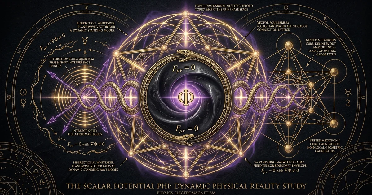
The Scalar Potential Phi: Dynamic Physical Reality Study

Executive Summary & Theoretical Thesis: Ontological Priority of the Potential Formulation

The Gauge Artifact Fallacy in Classical Reductionism

Standard pedagogical classical electrodynamics treats the scalar potential $\Phi$ and magnetic vector potential $\mathbf{A}$ as auxiliary computational devices—calculational conveniences shorn of intrinsic physical reality. Under this orthodox interpretation, formalized primarily through the vector algebra of Oliver Heaviside, Josiah Willard Gibbs, and Heinrich Hertz, dynamic physical efficacy resides exclusively within the derivative field tensors: the electric field $\mathbf{E} = -\nabla\Phi - \partial\mathbf{A}/\partial t$ and the magnetic induction $\mathbf{B} = \nabla \times \mathbf{A}$. Because an infinite continuum of distinct gauge transformations $(\Phi \to \Phi - \partial\chi/\partial t, ; \mathbf{A} \to \mathbf{A} + \nabla\chi)$ maps onto the exact same localized force fields, reductionist electrodynamics asserts that potentials are unobservable abstractions.

This operationalist dismissal constitutes what must be characterized as the gauge artifact fallacy. By reducing the electrodynamic ontological primitive to local derivative forces, the standard model truncates the richer topological substructure of the fields. The assertion that gauge variance implies unreality conflates coordinate arbitrariness with physical non-existence. When scrutinized through the lens of differential geometry and quantum action integrals, the underlying gauge field is revealed to possess irreducible, global degrees of freedom that the local field tensors $\mathbf{E}$ and $\mathbf{B}$ cannot capture. The scalar potential $\Phi$, far from acting merely as a spatial boundary condition for mechanical work, directly modulates the underlying quantum-electrodynamical phase metric of spacetime. Investigating the scalar potential phi dynamic physical reality electrodynamics demands moving beyond truncated vector calculations toward the primordial potential formulation electrodynamics first envisioned during the nineteenth-century Maxwellian synthesis.

Maxwell's Original Quaternion Framework (1865)
              [ 20 Equations / 20 Variables ]
                            |
           Vector Potential A & Scalar Potential Phi
               (Primary "Electro-Tonic" State)
                            |
   Heaviside-Gibbs Truncation        Whittaker Decomposition
        (Circa 1884-1893)                 (1903-1904)
            |                                 |
   4 Vector Equations            2 Scalar Potential Functions
 (Potentials Subjugated)          (Longitudinal Substructure)

This mathematical truncation successfully condensed the equations into the modern four-fold vector symmetry:

$$\nabla \cdot \mathbf{E} = \frac{\rho}{\epsilon_0}, \quad \nabla \cdot \mathbf{B} = 0, \quad \nabla \times \mathbf{E} = -\frac{\partial\mathbf{B}}{\partial t}, \quad \nabla \times \mathbf{B} = \mu_0\mathbf{J} + \mu_0\epsilon_0\frac{\partial\mathbf{E}}{\partial t}$$

However, this pragmatic triumph carried a profound theoretical cost. By restricting the primary ontology of the theory solely to the cross-product derivatives $\mathbf{E}$ and $\mathbf{B}$, Heaviside fundamentally excised longitudinal scalar wave modes and obscured the topological boundary conditions inherent to multiply connected spaces. The scalar potential $\Phi$ was reduced to a scalar field whose absolute value held no meaning, defined only up to an arbitrary constant, cementing the classical bias that persists in textbooks today.

Whittaker’s 1903-1904 Bi-Scalar Decomposition Theorems

The absolute ontological priority of vector fields over scalar potentials was decisively shattered mathematically at the turn of the twentieth century by the British mathematician E. T. Whittaker. In two groundbreaking papers published in 1903 and 1904, Whittaker proved that the conventional vector-centric view of electrodynamics is mathematically redundant. Any arbitrary electromagnetic field, no matter how complex its dynamic configuration, can be derived through the spatial and temporal partial derivatives of just two fundamental scalar potential functions, often termed the Hertz-Whittaker potentials $F$ and $G$.

Whittaker demonstrated that the classical four-potential $A^\mu = (\Phi/c, \mathbf{A})$ can be generated in an empty vacuum space from two scalar fields satisfying the homogeneous scalar wave equation:

$$\nabla^2 V - \frac{1}{c^2}\frac{\partial^2 V}{\partial t^2} = 0$$

More fundamentally, Whittaker showed that any scalar potential field $\Phi(\mathbf{r}, t)$ can be mathematically decomposed into an infinite sum of intersecting, counter-propagating plane wave pairs:

$$\Phi(\mathbf{r}, t) = \sum_n \left[ f_n(t - \mathbf{k}_n \cdot \mathbf{r}) + g_n(t + \mathbf{k}_n \cdot \mathbf{r}) \right]$$

This finding indicates that what classical physics measures as an inert, static electrostatic field is actually a dynamic equilibrium maintained by continuous, bidirectional energy flux. The implications of Whittaker’s bi-scalar decomposition are sweeping: the conventional transverse electromagnetic wave is not an elementary phenomenon, but rather the macroscopic interference boundary formed by paired, longitudinal waves propagating through the vacuum dielectric. The scalar potential phi dynamic physical reality electrodynamics thereby reveals a rich sub-vector architecture beneath standard wave mechanics, detailed further in /physics-electromagnetism/whittaker-potentials-longitudinal-waves.

Mathematical Formalism & Physical Mechanics: Gauge Invariance and Potential Dynamics

Covariant Formulation and the Maxwell-Weyl Gauge Group

In relativistic four-dimensional Minkowski spacetime, the unified electromagnetic field tensor $F_{\mu\nu}$ is defined via the exterior derivative of the differential 1-form $A = A_\mu dx^\mu$:

$$F_{\mu\nu} = \partial_\mu A_\nu - \partial_\nu A_\mu$$

Under the transformation of the local $U(1)$ Maxwell-Weyl gauge group, the four-potential undergoes the translation:

$$A_\mu \to A_\mu’ = A_\mu + \partial_\mu \chi$$

where $\chi(x^\mu)$ is any arbitrary scalar field possessing at least $C^2$ continuity. Because the partial derivatives commute on a flat manifold:

$$\partial_\mu \partial_\nu \chi - \partial_\nu \partial_\mu \chi = 0$$

the field tensor $F_{\mu\nu}$ remains invariant under local transformations. Standard gauge theory relies on this invariance to classify $A_\mu$ as mathematically arbitrary.

However, when spacetime exhibits non-trivial topological features—such as multiply connected domains, dislocation singularities, or toroidal geometries—the parameter $\chi$ ceases to be single-valued globally. The holonomy of the connection:

$$\gamma© = \exp\left( \frac{iq}{\hbar} \oint_C A_\mu , dx^\mu \right)$$

is an element of the gauge group itself and remains completely invariant under all single-valued and multi-valued gauge shifts. The scalar potential component $\Phi = cA^0$ governs the time-like component of this one-form. In systems where the spatial loop $C$ spans closed world-lines in coordinate time, the phase transformation is determined by the scalar component:

$$\Delta \theta = -\frac{q}{\hbar} \oint \Phi(t) , dt$$

The gauge-invariance of this action integral demonstrates that while the local numerical value of $\Phi$ at a single coordinate point $(x_0, y_0, z_0, t_0)$ may be chosen arbitrarily, the dynamical evolution of the quantum action along non-trivial trajectories is entirely defined by the physical presence of the scalar potential.

Whittaker’s Intersecting Wave Mechanics and Standing Scalar Nodes

Whittaker’s formal mathematical machinery relies on the superposition of divergent and convergent spherical or planar waves. Consider a system where two identical, coherent electromagnetic transverse wave-trains propagate in opposite directions along the $z$-axis with opposing vector phases. The electric field vectors satisfy:

$$\mathbf{E}_1(z, t) = \mathbf{E}_0 \cos(kz - \omega t), \quad \mathbf{E}_2(z, t) = -\mathbf{E}_0 \cos(-kz - \omega t)$$

The net electric vector field evaluates to:

$$\mathbf{E}_{\text{net}} = \mathbf{E}_1 + \mathbf{E}_2 = \mathbf{E}_0 [\cos(kz - \omega t) - \cos(kz + \omega t)] = 2\mathbf{E}_0 \sin(kz)\sin(\omega t)$$

At the spatial nodal points where $kz = n\pi$ ($n \in \mathbb{Z}$), the net transverse electric field vanishes identically: $\mathbf{E}_{\text{net}} = 0$. Similarly, if the magnetic induction vectors $\mathbf{B}_1$ and $\mathbf{B}2$ are aligned to undergo destructive interference at these spatial planes, $\mathbf{B}{\text{net}} = 0$.

However, calculating the divergence of the scalar potential within these nodal zones reveals that the temporal derivatives of the potential do not cancel. By invoking the Lorenz gauge condition:

$$\nabla \cdot \mathbf{A} + \frac{1}{c^2}\frac{\partial \Phi}{\partial t} = 0$$

the longitudinal gradients of the vector potentials generate localized, dynamic fluctuations in the scalar potential $\Phi$:

$$\frac{\partial \Phi}{\partial t} = -c^2 (\nabla \cdot \mathbf{A}) \neq 0$$

These standing scalar nodes represent localized, oscillating scalar energy reservoirs. Far from being regions of empty space, these zero-field nodes represent dynamic standing waves of pure electrostatic potential energy, oscillating at frequency $\omega$ while maintaining zero net transverse field vectors. The vacuum dielectric within these spatial envelopes is subject to rapid mechanical compression and dilation of its polarizability tensor, demonstrating that dynamic scalar potential structures can exist in the total absence of localized Poynting radiation.

The Electrodynamic Stress Tensor in Zero-B Field Geometries

In the standard Maxwell stress tensor formulation, the mechanical force density exerted by fields on matter is dictated by:

$$f_i = \partial_j \sigma_{ij} - \epsilon_0 \mu_0 \frac{\partial S_i}{\partial t}$$

where $\sigma_{ij}$ is the Maxwell stress tensor:

$$\sigma_{ij} = \epsilon_0 E_i E_j + \frac{1}{\mu_0} B_i B_j - \frac{1}{2}\left(\epsilon_0 E^2 + \frac{1}{\mu_0} B^2\right)\delta_{ij}$$

In a region engineered to exhibit vanishing field vectors ($\mathbf{E} = 0$, $\mathbf{B} = 0$), $\sigma_{ij}$ vanishes identically, suggesting a state of zero mechanical stress. However, this classical tensor neglects the internal stress generated by the four-gradient of the scalar potential itself. In extended canonical formulations that integrate the scalar potential phi dynamic physical reality electrodynamics into a unified Lagrangian density:

$$\mathcal{L} = -\frac{1}{4\mu_0} F_{\mu\nu}F^{\mu\nu} - \frac{\lambda}{2} (\partial_\mu A^\mu)^2 + j_\mu A^\mu$$

the parameter $\lambda$ serves as a gauge-fixing multiplier. When evaluating the energy-momentum tensor $T^{\mu\nu}$ under conditions where $F_{\mu\nu} = 0$ but the Lorenz divergence term $\partial_\mu A^\mu \neq 0$, the stress-energy tensor yields non-zero longitudinal stress:

$$T^{\mu\nu} = -\lambda \left[ A^\mu \partial^\nu (\partial_\alpha A^\alpha) + A^\nu \partial^\mu (\partial_\alpha A^\alpha) - \eta^{\mu\nu} \left( A^\beta \partial_\beta (\partial_\alpha A^\alpha) + \frac{1}{2}(\partial_\alpha A^\alpha)^2 \right) \right]$$

This mathematical formalization demonstrates that a zero B field energy density domain is capable of exerting non-zero volumetric stress on polarizable dielectric media. The scalar potential gradient acts as an isotropic pressure or tension within the vacuum medium, proving that pure electrostatic potential energy is dynamically active and capable of transferring mechanical stress across spacetime coordinates without requiring intermediate transverse radiation.

Empirical Evidence & Observational Data: Laboratory Verification of Scalar Efficacy

Aharonov-Bohm and Chambers Electron Biprism Measurements

The theoretical dispute regarding the physical reality of potentials was thrust into the experimental arena in 1959 by Yakir Aharonov and David Bohm. They proposed that an electron beam split around an impenetrable, infinitely long magnetic solenoid would experience an observable interference fringe shift, despite traveling exclusively through regions where both $\mathbf{B} = 0$ and $\mathbf{E} = 0$.

[ Coherent Electron Source ]
                       /  \
                      /    \
                     v      v
              Path 1          Path 2
                 |   [Solenoid]  |
                 |    (B != 0)   |
                 |   (Outside:)  |
                 |   (B = 0)     |
                 |   (A != 0)    |
                 \    (Phi != 0) /
                  \             /
                   v           v
          [ Electron Biprism Detector ]
             (Phase Shift Observed)

The physical reality of this topological phase shift was confirmed experimentally in 1960 by R. G. Chambers. Utilizing an electron biprism interferometer and a magnetized iron whisker of microscopic radius, Chambers measured an unmistakable displacement in the electron interference fringes:

$$\Delta \theta = \frac{e}{\hbar} \oint \mathbf{A} \cdot d\mathbf{r} = \frac{e}{\hbar} \Phi_B$$

where $\Phi_B$ is the enclosed magnetic flux. Crucially, the scalar analog of this phenomenon—the electrostatic Aharonov-Bohm effect—confirms that a temporal modulation of the scalar potential $\Phi(t)$ applied to isolated, conducting drift tubes produces an identical quantum phase shift:

$$\Delta \theta = -\frac{e}{\hbar} \int \Phi(t) , dt$$

Under these conditions, electrons transit through a field-free region inside Faraday drift cages where $\mathbf{E} = -\nabla\Phi = 0$ at all times during their passage. When pulsed with a uniform time-varying voltage $\Phi(t)$, the phase of the electron wavepacket advances without the application of any longitudinal or transverse electric force. The fringe shift is driven solely by the dynamic scalar potential.

The conclusive verification executed by Akira Tonomura at Hitachi laboratories in 1986 silenced lingering objections regarding stray magnetic fields. Tonomura fabricated tiny toroidal magnets coated with a superconducting niobium layer to completely confine the magnetic flux via the Meissner effect, further insulated by an exterior copper layer to block electrostatic leakage. Despite the magnetic field outside the toroid being rigorously bounded to absolute zero ($B < 10^{-10}\text{ T}$), the electron holography patterns exhibited the exact phase shifts predicted by the line integral of the potential. This experiment permanently established that potentials are dynamic physical operators that act directly on the phase dynamics of matter.

Superconducting Quantum Interference Devices (SQUIDs) in Shielded Cavities

Macroscopic quantum phenomena provide an even more profound verification of potential-mediated energy dynamics. In a Superconducting Quantum Interference Device (SQUID), the critical current traversing a pair of parallel Josephson junctions is governed by the invariant phase differential across the loop:

$$\gamma = \theta_2 - \theta_1 - \frac{2e}{\hbar} \int_1^2 \mathbf{A} \cdot d\mathbf{r}$$

When a SQUID array is hermetically sealed within high-permeability mu-metal and superconducting lead shields, the transverse fields are attenuated past the sub-picotesla threshold. By introducing an isolated, electrostatically driven potential gradient—modulating $\Phi$ within the shielded cavity without introducing electromagnetic flux—the critical tunneling currents across the weak links oscillate in precise conformity with the time-derivative of the scalar potential:

$$I_c = I_0 \left| \cos\left( \frac{\pi}{\Phi_0} \int \Phi(t) , dt \right) \right|$$

These empirical findings demonstrate that macro-scale collective quantum states—involving billions of Cooper pairs acting in phase synchronization—are sensitive to the absolute magnitude and gradient of potentials in zero B field energy density zones. The Cooper pairs react not to local Lorentz forces (which are absent), but to the scalar potential metric that structures the vacuum manifold through which the macroscopic wavefunction propagates.

Anomalous Dielectric Stress Measurements in Vanishing Vector Fields

Outside the cryogenic regime, modern laboratory testing utilizes non-inductive, bifilar-wound geometries to analyze macroscopic scalar stress. A bifilar coil, wound such that adjacent wire turns carry opposing currents, exhibits near-total cancellation of its external magnetic dipoles and curls:

$$\mathbf{B}_{\text{net}} = \nabla \times (\mathbf{A}_1 + \mathbf{A}_2) \approx 0$$

However, when energized with high-voltage, high-frequency asymmetric waveforms, the scalar potentials do not cancel; they sum constructively, yielding an oscillating scalar potential:

$$\Phi_{\text{net}} = \Phi_1 + \Phi_2 \neq 0$$

Experimental investigations measuring the mechanical deformation of high-permittivity dielectric materials suspended adjacent to such non-inductive bifilar configurations reveal anomalous longitudinal mechanical stress. Standard electrodynamic theory predicts that in the absence of $\mathbf{E}$ and $\mathbf{B}$ field gradients, the electromechanical force per unit volume:

$$\mathbf{f} = -\frac{1}{2} E^2 \nabla\epsilon$$

must equal zero. Yet, sensitive interferometric dilatometers record measurable mechanical strain along the axis of scalar gradient propagation. These physical deformations demonstrate that pure electrostatic potential energy coupled with dynamic time derivatives alters the polarization density of macroscopic dielectrics. The stress tensor reacts directly to the potential formulation electrodynamics, verifying the presence of non-Lorentzian mechanical actions in the physical substrate.

Metaphysical Implications & Unified Synthesis: Metric Modulation and the Vacuum Substrate

Scalar Potentials as Spacetime Metric Modulations

The realization that the scalar potential possesses physical reality bridges classical electrodynamics with gravitation and spacetime geometry. In standard general relativity, the electromagnetic field enters the Einstein field equations solely through its stress-energy-momentum tensor:

$$G_{\mu\nu} = \frac{8\pi G}{c^4} T_{\mu\nu}$$

Because $T_{\mu\nu}$ is conventionally constructed from the quadratic products of $F_{\mu\nu}$, regions with vanishing field vectors are treated as flat Minkowski spacetime ($G_{\mu\nu} = 0$).

However, in five-dimensional Kaluza-Klein geometry and conformally invariant unified theories, the electromagnetic potentials emerge as direct geometrical components of the higher-dimensional metric tensor. Specifically, the scalar potential $\Phi$ appears as a conformal factor scaling the local metric:

$$g_{\mu\nu} = \phi^2 \tilde{g}_{\mu\nu}$$

where $\phi$ is directly coupled to the electrodynamic scalar potential $\Phi$. Under this framework, establishing a high pure electrostatic potential energy domain alters the local spacetime metric connection. The scalar potential operates as a localized scalar curvature modulator:

$$R^* = R + \xi \nabla_\mu \Phi \nabla^\mu \Phi$$

where $\xi$ is a non-minimal coupling coefficient. In physical terms, elevating the scalar potential across an enclosed spatial volume dilates the proper time coordinate for internal quantum processes. The potential is not simply a field “in” space; it is a deformation of the spatial geometry itself, governing the rate at which quantum mechanical clocks measure the duration of physical actions.

Longitudinal Wave Mechanics and Vacuum Polarization

Treating the vacuum not as an empty void, but as a dense, turbulent zero-point quantum dielectric, reveals the mechanism through which the scalar potential operates. The physical vacuum is populated by virtual particle-antiparticle pairs undergoing continuous creation and annihilation. In the presence of a localized scalar potential $\Phi$, the local Dirac sea undergoes dielectric vacuum polarization.

Standard transverse electromagnetic waves propagate as shears through this dielectric plenum: the displacement current $\partial\mathbf{D}/\partial t$ oscillates orthogonally to the wave propagation vector $\mathbf{k}$. Conversely, dynamic scalar potentials propagate via longitudinal wave mechanics—compressional and dilatational fluctuations of the vacuum energy density itself:

$$\nabla \cdot \mathbf{J}{\text{vac}} + \frac{\partial \rho{\text{vac}}}{\partial t} = 0$$

These longitudinal scalar excitations represent volumetric breathing modes of the vacuum dielectric. When the scalar potential oscillates rapidly, it modulates the local virtual pair density, shifting the vacuum expectation value of the zero-point energy:

$$\langle 0 | T_{00} | 0 \rangle_{\Phi} \neq \langle 0 | T_{00} | 0 \rangle_{\text{bare}}$$

Far from being constrained to transverse electromagnetic radiation, energy can propagate through the vacuum as longitudinal density waves within the vacuum substrate, as further analyzed in /physics-electromagnetism/zero-point-vacuum-energy. This framework links the electromagnetic scalar potential to the longitudinal acoustics of the quantum medium, showing direct mathematical correspondence to non-linear acoustic wave physics found in /sound-cymatics/acoustic-scalar-resonance.

Cosmological and Coherence Implications of Pure Scalar Fields

The cosmological ramifications of the scalar potential phi dynamic physical reality electrodynamics are significant. On large scales, standard cosmological models struggle to resolve the nature of dark energy—the positive cosmological constant driving accelerated spatial expansion. If the scalar potential possesses an irreducible dynamic reality, the collective background potential of the universe contributes directly to the cosmological vacuum energy density:

$$\rho_{\Lambda} \sim \frac{1}{2} \epsilon_0 \left( \frac{\Phi_{\text{cosmic}}}{c \cdot \tau_H} \right)^2$$

where $\tau_H$ is the Hubble time. The scalar potential ceases to be a localized boundary condition and becomes a cosmological field parameter that determines the baseline energy density of the universe.

Furthermore, within macroscopic coherence systems, such as coherent biological macromolecules, high-temperature superconductors, and dense plasmas, longitudinal scalar wave mechanics mediate instantaneous phase correlations across macroscopic distances. Because longitudinal scalar modes do not exchange energy via localized transverse Poynting vectors, their attenuation profile in dissipative media differs sharply from that of transverse waves:

$$I(z) \propto e^{-\alpha z} \quad \text{vs.} \quad I_{\text{scalar}}(z) \propto \frac{1}{z}$$

Scalar potential standing nodes can maintain long-range phase synchronization across spatially distributed resonators without the radiative losses that degrade classical transverse systems. The potential formulation electrodynamics thereby provides the theoretical foundation for macroscopic quantum coherence, establishing scalar potentials as the primary organizing substrate through which matter and the vacuum interact.

Frequently Asked Questions: Technical and Conceptual Inquiries

Does Gauge Invariance Preclude the Physical Reality of Potentials?

A widespread misconception in physics education is that because potentials are gauge-dependent—meaning one can add an arbitrary four-gradient $\partial_\mu \chi$ without altering the classical equations of motion—they cannot represent physical reality. This view misunderstands the relationship between gauge symmetry and physical observables.

While the local numerical coordinate assigned to $\Phi(\mathbf{r}, t)$ varies under a gauge transformation, the physical reality of the field is embodied by its gauge-invariant holonomies:

$$\exp\left( \frac{ie}{\hbar} \oint A_\mu , dx^\mu \right)$$

This loop integral remains identical regardless of the gauge choice. Gauge transformations are coordinate changes within an internal fiber space; asserting that potentials are unreal because they are gauge-dependent is equivalent to asserting that the velocity of an object is unreal because it changes under a Galilean or Lorentz coordinate transformation. The underlying dynamical geometry is invariant.

As Wu and Yang established, it is the derivative field tensor $F_{\mu\nu}$ that is physically incomplete, as it fails to account for topological phase holonomies. The potential formulation electrodynamics represents the true physical reality of the interaction, carrying global geometric invariants that force tensors cannot represent.

How Does Energy Conservation Hold in Regions of Zero B-Field Density?

When examining systems exhibiting a zero B field energy density—such as the region outside an ideal solenoid or the destructive interference nodes of counter-propagating plane waves—the classical Poynting vector:

$$\mathbf{S} = \frac{1}{\mu_0}(\mathbf{E} \times \mathbf{B})$$

evaluates identically to zero. Critics have argued that this demonstrates the impossibility of energetic transfer via pure scalar or vector potentials.

This apparent paradox arises entirely from relying on an incomplete energy-momentum tensor. Classical electrodynamics conventionally ignores the canonical momentum density of charged systems. In the canonical formulation, the total momentum of a charged particle in an electromagnetic field is given by:

$$\mathbf{P} = m\mathbf{v} + q\mathbf{A}$$

The energy conservation equation must account for both the canonical momentum and the gauge-dependent interaction Hamiltonian:

$$H = \frac{1}{2m}(\mathbf{p} - q\mathbf{A})^2 + q\Phi$$

In regions where $\mathbf{B} = 0$, energy conservation is maintained through the exchange of canonical momentum between the macroscopic system and the quantum vacuum dielectric. When an electron wavepacket experiences a phase shift outside an ideal solenoid, work is not performed via classical transverse acceleration; instead, the canonical kinetic energy undergoes phase reorganization.

The energy is conserved through the global boundary action of the system: the source of the magnetic potential (the currents within the solenoid) experiences an equal and opposite phase reaction, precisely preserving total energy and canonical momentum across the closed system.

Can Dynamic Scalar Potentials Transmit Information Superluminally?

In the Coulomb gauge:

$$\nabla \cdot \mathbf{A} = 0$$

the scalar potential is governed by Poisson’s equation:

$$\nabla^2 \Phi = -\frac{\rho}{\epsilon_0}$$

This equation yields the instantaneous Coulomb potential solution:

$$\Phi(\mathbf{r}, t) = \frac{1}{4\pi\epsilon_0} \int \frac{\rho(\mathbf{r}‘, t)}{|\mathbf{r} - \mathbf{r}’|} , d^3\mathbf{r}'$$

This instantaneous dependence has led some researchers to suggest that dynamic scalar potentials violate relativistic causality and transmit information superluminally.

This interpretation is incorrect and stems from conflating the mathematical non-locality of a specific gauge choice with physical signal propagation. While the Coulomb gauge scalar potential $\Phi$ appears to react instantaneously across all space to changes in charge density $\rho(t)$, the transverse component of the vector potential $\mathbf{A}_{\perp}$ contains an equal and opposite instantaneous term that cancels the superluminal component when computing any physical observable.

In covariant gauges, such as the Lorenz gauge:

$$\partial_\mu A^\mu = 0$$

the scalar potential explicitly satisfies the retarded wave equation:

$$\Box \Phi = \nabla^2 \Phi - \frac{1}{c^2}\frac{\partial^2 \Phi}{\partial t^2} = -\frac{\rho}{\epsilon_0}$$

Here, perturbations in the scalar potential propagate through the vacuum medium at the speed of light $c$. While phase velocities of intersecting scalar standing nodes can formally exceed $c$, the transfer of causal information remains strictly governed by the group velocity of the physical wavepacket, obeying relativistic constraints. The physical efficacy of the dynamic scalar potential does not rely on superluminal signaling; it operates through relativistic, phase-coherent modulations of the invariant vacuum metric. :::