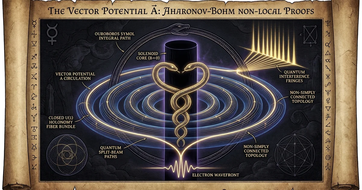
The Vector Potential A: Aharonov-Bohm Non-Local Proofs
Executive Summary & Theoretical Thesis
The Classical Field Ontology vs. Quantum Gauge Realism
In classical electrodynamics as synthesized by the Maxwell-Heaviside equations, physical reality is assigned exclusively to the local force fields: the electric field $\mathbf{E}$ and the magnetic field $\mathbf{B}$. Within this Newtonian and Cartesian paradigm, the magnetic vector potential $\mathbf{A}$ and the electric scalar potential $\Phi$ are traditionally dismissed as auxiliary mathematical variables. They are understood as unphysical computational artifacts introduced to exploit the differential identities $\nabla \cdot \mathbf{B} = 0$ (implying $\mathbf{B} = \nabla \times \mathbf{A}$) and $\nabla \times \mathbf{E} = -\partial \mathbf{B}/\partial t$ (implying $\mathbf{E} = -\nabla\Phi - \partial\mathbf{A}/\partial t$). Because $\mathbf{A}$ admits infinite gauge freedom under the local transformation $\mathbf{A} \rightarrow \mathbf{A} + \nabla\Lambda$, classical ontology assumes that arbitrary, gauge-dependent parameters cannot directly exert dynamical influence upon physical matter. Contact action, mediated strictly by local field tensors $F_{\mu\nu}$ via the Lorentz force law $\mathbf{F} = q(\mathbf{E} + \mathbf{v} \times \mathbf{B})$, stands as the defining postulate of classical local realism.
Quantum gauge realism systematically dismantles this reductionist framework. The fundamental interaction Hamiltonian of an electrically charged quantum particle does not couple to field tensors through local differential forces. Instead, it couples directly to the four-potential $A_\mu = (\Phi/c, -\mathbf{A})$ through the canonical momentum operator $\mathbf{P} = \mathbf{p} - q\mathbf{A}$. The emergence of the Aharonov-Bohm effect proves that particles moving through space where local field strengths vanish identically ($\mathbf{B} = 0$, $\mathbf{E} = 0$, hence $F_{\mu\nu} = 0$) nonetheless accumulate an observable, gauge-invariant phase shift. This interaction isolates the vector potential $\mathbf{A}$ as an ontologically primary field quantity, refuting the classical premise that potentials are merely arbitrary computational devices.
Classical Maxwell-Heaviside Paradigm
- Primary Ontology: Local force fields $\mathbf{E}(x, t)$ and $\mathbf{B}(x, t)$ defined as physically real vectors at every spacetime point.
- Status of Potentials: Auxiliary computational contrivances; unmeasurable gauge artifacts possessing no independent physical reality.
- Locality Mechanism: Strict contact action governed by the Lorentz force law $\mathbf{F} = q(\mathbf{E} + \mathbf{v} \times \mathbf{B})$; interactions require local field strength tensors $F_{\mu\nu} \neq 0$.
- Space Topology: Trivial Euclidean $\mathbb{R}^3$ or Minkowski $\mathbb{M}^4$; topological defects or multiply connected regions do not alter local dynamics.
Quantum Topological Gauge Paradigm
- Primary Ontology: Connection forms $A_\mu$ on a principal $U(1)$ bundle, whose closed-loop path integrals define non-integrable phase factors.
- Status of Potentials: Fundamentally real; local field strengths $F_{\mu\nu}$ represent derived extrinsic curvatures of the underlying connection.
- Locality Mechanism: Quantum non-locality mediated by topological holonomies; actions occur where classical field tensors strictly vanish ($F_{\mu\nu} = 0$).
- Space Topology: Non-simply connected manifolds $\mathcal{M}$; physical observables correspond to global topological invariants and de Rham cohomology classes.
Topological Invariants and the Non-Simply Connected Vacuum
The physical reality of potentials is intimately coupled to the topology of the underlying configuration space. When an infinite cylinder of magnetic flux $\Phi$ is established in an otherwise field-free vacuum, the physical space accessible to propagating charged wavefunctions becomes topologically non-trivial. The spatial manifold is no longer simply connected; it degenerates into a multiply connected manifold topologically homeomorphic to $\mathbb{R}^3 \setminus S^1$, possessing a non-trivial first fundamental group: $$\pi_1(\mathcal{M}) \cong \mathbb{Z}$$
In this non-simply connected vacuum, paths that encircle the excluded magnetic domain cannot be continuously deformed to a point without passing through the singularity where $F_{\mu\nu} \neq 0$. Consequently, closed-loop line integrals of the connection form along topologically distinct homotopy classes yield invariant non-zero phases. This behavior establishes that the vector potential $\mathbf{A}$, while locally flat ($\nabla \times \mathbf{A} = 0$), carries a global topological invariant. The vacuum state itself acquires non-trivial geometrical structure, demonstrating that quantum dynamics depends on global topological context rather than solely on localized field forces. This interaction reveals that electromagnetic forces are merely the local curvatures of a much deeper, globally connected gauge-invariant quantum topology.
The Paradigm Shift: From Local Force Vectors to Global Phase Holonomies
This empirical and theoretical divergence marks a transition from Newtonian point-mechanics to global holonomy physics. The Aharonov-Bohm effect provides definitive non-local quantum proof that physical states depend on non-integrable phase factors: $$W(\gamma) = \mathcal{P} \exp \left( \frac{i q}{\hbar} \oint_\gamma A_\mu , dx^\mu \right)$$ These Wilson loops act as global operators across the manifold.
The measurable shift in quantum interference patterns without a localized magnetic field ($\mathbf{B} = 0$) demonstrates that physical systems evaluate the global topological structure of the gauge bundle along their complete trajectories. Action-at-a-distance is not mediated by instantaneous classical signaling, but rather by the non-local integration of the gauge connection across the entire phase space of the wavefunction. This shift demands a radical reconsideration of the vacuum substrate, requiring mathematical tools drawn from differential geometry, fiber bundles, and de Rham cohomology to supplant the limited vector calculus of nineteenth-century field theory.
Historical Lineage & Experimental Precedents
Maxwell’s Electrotonic State and the Heaviside Reduction
The status of the vector potential $\mathbf{A}$ has been a point of debate since the inception of field theory. In his seminal 1865 treatise, A Dynamical Theory of the Electromagnetic Field, James Clerk Maxwell established the foundation of electrodynamics around an entity he termed the “electrotonic state.” This fundamental dynamical quantity was represented by the vector potential $\mathbf{A}$. Maxwell considered the electrotonic state to be an actual mechanical momentum stored within the underlying electromagnetic ether, from which electric and magnetic intensities were derived via spatial and temporal derivatives.
Following Maxwell’s death, the “Maxwellians”—principally Oliver Heaviside, Heinrich Hertz, and Josiah Willard Gibbs—sought to cleanse the theory of what they perceived as superfluous metaphysical baggage and unobservable mechanical variables. Heaviside, aggressively reformulating Maxwell’s original twenty quaternion equations into four vector equations, excised the electrotonic state from fundamental status. He argued that because $\mathbf{A}$ could be altered by adding the gradient of an arbitrary scalar function without altering the forces exerted on classical test charges, it represented an unphysical mathematical scaffolding. This Heaviside reduction codified the classical orthodoxy: force fields $\mathbf{E}$ and $\mathbf{B}$ were elevated to primary physical realities, while the potential potentials $\mathbf{A}$ and $\Phi$ were relegated to auxiliary conveniences. The historic implications of this mathematical purge are analyzed extensively in the study of /physics-electromagnetism/maxwell-quaternions-lost-terms, which details how higher-order communicative vacuum components were systematized out of nineteenth-century electrodynamics.
Primary Literature Sources:
- Maxwell, J. C. (1865). “A Dynamical Theory of the Electromagnetic Field.” Philosophical Transactions of the Royal Society of London, 155, 459–512.
- Maxwell designates the vector potential $\mathbf{A}$ as the primary dynamical variable: “The electrotonic state is the fundamental quantity in the theory of electricity… it represents the total electromagnetic momentum of the system.”
- Aharonov, Y., & Bohm, D. (1959). “Significance of Electromagnetic Potentials in the Quantum Theory.” Physical Review, 115(3), 485–491.
- Aharonov and Bohm establish the fundamental quantum status of potentials: “Contrary to the conclusions of classical mechanics, there exist effects of potentials on charged particles, even in the region where all the field strengths (and consequently the forces on the particles) vanish.”
The Ehrenberg-Siday 1949 Precursor and the Aharonov-Bohm 1959 Paper
A decade prior to the famous work of Yakir Aharonov and David Bohm, an optical formulation of this topological effect was derived by Werner Ehrenberg and Raymond E. Siday. In their 1949 paper, “The Refractive Index in Electron Optics and the Principles of Dynamics,” published in the Proceedings of the Physical Society, Ehrenberg and Siday applied the de Broglie-Fermat optical path principle to electron beams traversing magnetic systems. They noted that the effective quantum refractive index: $$\mu = \sqrt{1 - \frac{2mqV}{p^2}} + \frac{q}{p} (\mathbf{A} \cdot \mathbf{t})$$ inevitably produced a spatial phase shift when electron wavepackets were routed around an enclosed magnetic flux, even if the wavepackets experienced no local magnetic field along their trajectory.
Ehrenberg and Siday’s pioneering calculation went largely unnoticed, framed as it was within the narrow technical literature of electron microscope objective aberrations. It was not until 1959 that Yakir Aharonov and David Bohm, working at the University of Bristol, independently rediscovered this phenomenon and formulated its comprehensive quantum mechanical and epistemological implications. Aharonov and Bohm recognized that this was not merely a lens aberration, but a profound breakdown of classical field ontology. They demonstrated that the non-integrable phase factor acquired by the wavefunction across a field-free multiply connected domain demonstrated the physical reality of potentials, forcing physics to abandon its strict adherence to local classical force vectors.
Early Experimental Controversies and the Classical Leakage Critique
The publication of the 1959 paper catalyzed intense debate within the theoretical and experimental physics communities. Classical determinists and orthodox field theorists, reluctant to accept non-local phase actions, claimed that the observed effects were experimental artifacts. The principal critique was the “classical leakage hypothesis,” championed by theorists such as F. T. Eaton and P. Bocchieri. They argued that any real solenoid of finite length inherently radiates fringe dipole and quadrupole magnetic fields into the exterior zone. Therefore, the electrons were simply interacting with minute, classical Lorentz force fields ($q\mathbf{v} \times \mathbf{B}_{\text{leakage}} \neq 0$) rather than responding to a non-local vector potential.
This skepticism led to decades of high-precision micro-interferometric experiments. Early attempts using macroscopic wire coils, magnetized whiskers, and micro-solenoids struggled to eliminate fringing fields down to the quantum limit. The controversy underscored the necessity of designing an experimental geometry in which the magnetic flux was rigorously, provably, and topologically enclosed within an impenetrable superconducting shield. This experimental demand would not be met until the microfabrication breakthroughs of the mid-1980s.
Mathematical Formalism & Physical Mechanics
The Non-Integrable Phase Factor and Dirac Path Integrals
To understand the mechanics of the Aharonov-Bohm effect, consider the Feynman path-integral formulation of quantum mechanics. The transition amplitude $K(b, a)$ for an electron of mass $m$ and charge $q = -e$ propagating from point $a$ to point $b$ is given by the functional sum over all kinematically accessible trajectories $\gamma$: $$K(b, a) = \int \mathcal{D}[\mathbf{x}(t)] \exp\left(\frac{i}{\hbar} S[\mathbf{x}(t)]\right)$$ In the presence of an external electromagnetic potential $A_\mu = (\Phi/c, -\mathbf{A})$, the classical action $S[\mathbf{x}(t)]$ incorporates the minimal coupling Lagrangian: $$L = L_0 + L_{\text{int}} = \frac{1}{2}m\mathbf{v}^2 + q(\mathbf{A} \cdot \mathbf{v}) - q\Phi$$
The total action along any specific trajectory $\gamma$ separates into a field-free kinematic component $S_0[\gamma]$ and an electromagnetic phase component $S_{\text{EM}}[\gamma]$: $$S[\gamma] = \int_{t_a}^{t_b} L_0 , dt + q \int_{t_a}^{t_b} (\mathbf{A} \cdot \dot{\mathbf{x}} - \Phi) , dt = S_0[\gamma] + q \int_\gamma (\mathbf{A} \cdot d\mathbf{r} - \Phi , dt)$$
When the electrostatic scalar potential vanishes ($\Phi = 0$) and the magnetic field along the trajectory is zero ($\mathbf{B} = \nabla \times \mathbf{A} = 0$), the wavefunctions along paths $\gamma_1$ and $\gamma_2$ traversing opposite sides of an enclosed, shielded flux domain acquire a non-integrable Dirac phase factor. The respective probability amplitudes superpose at the detector: $$\psi_{\text{total}} = \psi_1 + \psi_2 = \psi_1^{(0)} \exp\left( \frac{i q}{\hbar} \int_{\gamma_1} \mathbf{A} \cdot d\mathbf{r} \right) + \psi_2^{(0)} \exp\left( \frac{i q}{\hbar} \int_{\gamma_2} \mathbf{A} \cdot d\mathbf{r} \right)$$ The resulting interference intensity $I \propto |\psi_{\text{total}}|^2$ depends fundamentally on the relative phase difference: $$\Delta\phi = \frac{q}{\hbar} \int_{\gamma_1} \mathbf{A} \cdot d\mathbf{r} - \frac{q}{\hbar} \int_{\gamma_2} \mathbf{A} \cdot d\mathbf{r} = \frac{q}{\hbar} \oint_{\Gamma} \mathbf{A} \cdot d\mathbf{r}$$ where $\Gamma = \gamma_1 - \gamma_2$ is the oriented, closed contour surrounding the inaccessible flux domain.
Consider the fundamental gauge transformation applied to the potentials: $$\mathbf{A}‘(\mathbf{r}, t) = \mathbf{A}(\mathbf{r}, t) + \nabla \Lambda(\mathbf{r}, t), \quad \Phi’(\mathbf{r}, t) = \Phi(\mathbf{r}, t) - \frac{\partial \Lambda(\mathbf{r}, t)}{\partial t}$$ Under this transformation, the electromagnetic interaction action along a trajectory $\gamma$ transforms as: $$S’{\text{EM}}[\gamma] = q \int\gamma \left[ \left(\mathbf{A} + \nabla \Lambda\right) \cdot d\mathbf{r} - \left(\Phi - \frac{\partial \Lambda}{\partial t}\right) dt \right] = S_{\text{EM}}[\gamma] + q \int_\gamma d\Lambda = S_{\text{EM}}[\gamma] + q \left[ \Lambda(b) - \Lambda(a) \right]$$ The local quantum mechanical wavefunction transforms simultaneously via the $U(1)$ local phase rotation: $$\psi’(\mathbf{r}, t) = \psi(\mathbf{r}, t) \exp\left( \frac{i q}{\hbar} \Lambda(\mathbf{r}, t) \right)$$ Thus, for an open path, the phase factor $\exp\left( \frac{i q}{\hbar} \int_a^b \mathbf{A} \cdot d\mathbf{r} \right)$ is explicitly gauge-dependent and unphysical on its own.
However, when evaluated over a closed loop $\Gamma$ ($a = b$), the boundary terms cancel completely: $$\oint_\Gamma \nabla \Lambda \cdot d\mathbf{r} = 0 \implies \Delta\phi’ = \frac{q}{\hbar} \oint_\Gamma \mathbf{A}’ \cdot d\mathbf{r} = \frac{q}{\hbar} \oint_\Gamma \mathbf{A} \cdot d\mathbf{r} = \Delta\phi$$ By application of Stokes’ theorem over the non-simply connected 2-surface $\Sigma$ bounded by $\partial\Sigma = \Gamma$: $$\Delta\phi = \frac{q}{\hbar} \iint_\Sigma (\nabla \times \mathbf{A}) \cdot d\mathbf{S} = \frac{q}{\hbar} \iint_\Sigma \mathbf{B} \cdot d\mathbf{S} = \frac{q}{\hbar} \Phi_B$$ This confirms that the relative phase shift without a local $\mathbf{B}$ field along the particle’s trajectory is strictly gauge-invariant and determined by the enclosed topological magnetic flux $\Phi_B$.
Gauge Invariance via Stokes’ Theorem and Holonomy Groups
The mathematical physics of this phenomenon was brought to modern maturity by Tai Tsun Wu and Chen Ning Yang in their seminal 1975 treatise. The Wu-Yang dictionary demonstrates that neither the local field tensor $F_{\mu\nu}$ nor the local gauge potential $A_\mu$ provides an intrinsic description of electromagnetism. The field tensor $F_{\mu\nu}$ underdescribes reality because it yields $F_{\mu\nu} = 0$ in the exterior region, failing to predict the phase shift. Conversely, the four-potential $A_\mu$ overdescribes reality because it introduces redundant, unmeasurable gauge freedoms.
The minimal, complete, and intrinsic description of electromagnetism is provided by the non-integrable phase factor: $$W(\Gamma) = \exp\left( \frac{i q}{\hbar} \oint_\Gamma A_\mu , dx^\mu \right)$$ Geometrically, this quantity is the holonomy of a principal fiber bundle with base space manifold $\mathcal{M}$ and structure group $G = U(1)$. The potential 1-form $A = A_\mu dx^\mu$ acts as a differential connection on this bundle. While the curvature 2-form: $$F = dA = \frac{1}{2} F_{\mu\nu} dx^\mu \wedge dx^\nu$$ vanishes throughout the region accessible to the particle, the holonomy group remains non-trivial because the base manifold is multiply connected. The loop $\Gamma$ belongs to a non-contractible homotopy class in $\pi_1(\mathcal{M})$. Thus, the phase shift without a local $\mathbf{B}$ field constitutes an unambiguous measurement of the global holonomy group of the gauge bundle. These concepts directly correlate to the harmonic dynamics detailed in /sound-cymatics/modal-topology-phase-resonance, where spatial boundary conditions generate distinct topological modes.
Schrödinger and Pauli Wave Equation Coupling to the Gauge Field
To trace the continuous evolution of this phase, consider the time-dependent Schrödinger equation coupled via minimal substitution: $$\frac{1}{2m} \left( -i\hbar\nabla - q\mathbf{A}(\mathbf{r}) \right)^2 \psi(\mathbf{r}, t) = i\hbar \frac{\partial \psi(\mathbf{r}, t)}{\partial t}$$ In a spatial domain where $\mathbf{B} = \nabla \times \mathbf{A} = 0$, we can express the vector potential locally as the gradient of a scalar field: $$\mathbf{A}(\mathbf{r}) = \nabla S(\mathbf{r})$$ This scalar function is multivalued over the entire multiply connected manifold: $$S(\mathbf{r}) = \int_{\mathbf{r}_0}^\mathbf{r} \mathbf{A}(\mathbf{r}‘) \cdot d\mathbf{r}’$$ We can apply a local gauge transformation to remove $\mathbf{A}$ from the differential equation by defining: $$\psi(\mathbf{r}, t) = \psi^{(0)}(\mathbf{r}, t) \exp\left( \frac{i q}{\hbar} S(\mathbf{r}) \right)$$ Substitution reveals that $\psi^{(0)}(\mathbf{r}, t)$ satisfies the entirely field-free Schrödinger equation: $$-\frac{\hbar^2}{2m} \nabla^2 \psi^{(0)}(\mathbf{r}, t) = i\hbar \frac{\partial \psi^{(0)}(\mathbf{r}, t)}{\partial t}$$
However, because the integral $S(\mathbf{r})$ depends on the topological winding number of the path taken from $\mathbf{r}_0$ to $\mathbf{r}$, the wavefunction $\psi(\mathbf{r}, t)$ cannot be globally single-valued unless it accounts for the topological phase accumulated around the boundary. If the particle possesses spin, the Pauli equation: $$\left[ \frac{1}{2m} \left( \boldsymbol{\sigma} \cdot \left( \mathbf{p} - q\mathbf{A} \right) \right)^2 + q\Phi \right] \Psi = i\hbar \frac{\partial \Psi}{\partial t}$$ collapses to the same scalar holonomic phase shift, demonstrating that the Aharonov-Bohm effect is fundamentally independent of spin-magnetic dipole interactions ($-\boldsymbol{\mu} \cdot \mathbf{B} = 0$) and stems strictly from orbital gauge dynamics.
Empirical Evidence & Observational Data
Chambers’ 1960 Whiskered Solenoid Interferences
The first experimental validation of the Aharonov-Bohm prediction was achieved by R. G. Chambers in 1960 at the University of Bristol. Chambers adapted an electron interferometer featuring an electrostatic biprism developed by Möllenstedt and Düker. In the shadow region behind the central biprism wire, Chambers positioned an iron magnetic whisker approximately $1,\mu\text{m}$ in diameter and several millimeters long. The whisker acted as a magnetized micro-cylinder, directing enclosed magnetic flux perpendicular to the split electron trajectories.
By tracking the interference fringes on an imaging plate, Chambers measured a fringe displacement corresponding directly to: $$\Delta x = \frac{\lambda L}{2\pi d} \left( \frac{e}{\hbar} \Phi_{\text{whisker}} \right)$$ where $\lambda$ represents the relativistic de Broglie wavelength of the accelerated electrons, $L$ is the optical baseline distance, and $d$ is the path separation. While Chambers confirmed the theoretical phase shift within experimental margins of error, skeptics highlighted the lack of absolute magnetic isolation. The tapered morphology of the iron whisker inherently permitted residual classical leakage flux to escape from its ends, sustaining the classical leakage critique.
Tonomura’s 1986 Toroidal Superconducting Magnet Experiments
The definitive experimental proof of the Aharonov-Bohm effect was executed in 1986 by Akira Tonomura and his research team at the Hitachi Advanced Research Laboratory. Tonomura recognized that to silence the leakage critique, the magnetic flux must be isolated behind an impenetrable physical barrier using superconductivity.
Source: Tonomura, A., Osakabe, N., Matsuda, T., Kawasaki, T., Endo, J., Yano, S., & Yamada, H. (1986). “Evidence for Aharonov-Bohm effect with magnetic field completely shielded by a superconductor.” Physical Review Letters, 56(8), 792–795.
- Electron Energy: $150,\text{keV}$ (Relativistic wavelength $\lambda_e = 3.0,\text{pm}$).
- Core Material: Ferromagnetic Permalloy ($\text{Fe}{0.19}\text{Ni}{0.81}$) torus with inner radius $r_1 = 2.5,\mu\text{m}$, outer radius $r_2 = 4.5,\mu\text{m}$, and thickness $t = 200,\text{nm}$.
- Inner Insulating Layer: Silicon Nitride ($\text{Si}_3\text{N}_4$) and Copper isolation coat, $100,\text{nm}$ thickness, preventing electron penetration into the magnet core.
- Superconducting Meissner Shield: Niobium ($\text{Nb}$) outer cladding, thickness $300,\text{nm}$, operating at critical temperature $T_c = 9.2,\text{K}$.
- Observed Fringe Shift: Step-function phase displacement of precisely $\pi$ radians across the inner and outer boundaries at magnetic flux quantization: $$\Delta\phi = \pi \pmod{2\pi}$$ Leakage magnetic field measured outside the superconductor: $|\mathbf{B}_{\text{leakage}}| < 10^{-6},\text{Gauss}$, eliminating classical Lorentz interactions.
Tonomura employed transmission electron holography to measure the interference fringes. A coherent $150,\text{keV}$ electron beam was split into two components via an electrostatic biprism: one beam traversed the central hole of the toroidal magnet, while the reference beam passed exterior to the toroid. At temperatures well below the $9.2,\text{K}$ critical threshold of Niobium, the Meissner effect expelled all residual flux from the superconductor. Because the London penetration depth of Niobium ($\lambda_L \approx 39,\text{nm}$) was small compared to the $300,\text{nm}$ shielding thickness, the exterior magnetic field dropped to zero.
The resulting holographic interferograms revealed a sharp, discontinuous step-function displacement in the fringe pattern traversing the ring’s interior hole versus its exterior perimeter. The phase shift coincided with the theoretical gauge-invariant flux integral, providing clear, non-local quantum proof that phase accumulation occurs in regions devoid of magnetic fields ($\mathbf{B} = 0$).
[ Electron Biprism Beam Source ]
              |
      +-------+-------+
      |               |
   [Path 1]        [Path 2]
      |               |
      |   +-------+   |
      |   | [Nb]  |   |
      |   | [Mag] |   |   <-- Meissner Shielded Toroid (B=0 outside)
      |   | [Nb]  |   |
      |   +-------+   |
      |               |
      +-------+-------+
              |
     [Interferogram Shift: Delta phi = q/hbar * Phi]
Modern Nanoscale Rings and Mesoscopic Aharonov-Bohm Oscillations
In modern condensed matter physics, the vector potential’s physical reality is demonstrated through Aharonov-Bohm oscillations in mesoscopic normal-metal and semiconductor rings (e.g., Gallium Arsenide/Aluminum Gallium Arsenide heterostructures). At sub-Kelvin temperatures, the phase coherence length $L_\phi$ of conduction electrons exceeds the micrometric circumference $L$ of the lithographically fabricated ring. When a magnetic field threads the ring’s center, the magnetoconductance $G$ across the ring oscillates periodically as a function of the threading magnetic flux: $$G(B) = G_0 + \sum_{n=1}^\infty G_n \cos\left( 2\pi n \frac{\Phi}{\Phi_0} \right)$$ where $\Phi_0 = h/e$ represents the normal electron flux quantum, and $\Phi_0’ = h/2e$ denotes the Altshuler-Aronov-Spivak (AAS) oscillation period arising from time-reversed backscattering paths.
These oscillations emerge because the vector potential modifies the complex quantum transfer matrix elements of electrons propagating through the ring arms. Even when the physical wire structure contains negligible internal magnetic flux, the non-local connection form $A_\mu$ shifts the constructive and destructive interference conditions for electron transmission, altering the sample’s macroscopic electrical resistance. The study of /sacred-geometry/topological-invariants-toroidal-fields highlights how these toroidal and annular geometries mirror fundamental topological invariants found in broader physical systems.
Metaphysical Implications & Unified Synthesis
EPR Paradox, Non-Locality, and the Demise of Cartesian Relationalism
The empirical reality of the Aharonov-Bohm effect exposes profound fractures within the classical metaphysics of space, matter, and causality. Under Cartesian relationalism, physical interactions are mediated by continuous, local, point-to-point mechanical forces. A particle cannot be influenced by an event or object unless the object’s localized force carrier makes direct physical contact with the particle: $$F_{\mu\nu}(x) \neq 0, \quad x \in \text{supp}(\psi)$$ The Aharonov-Bohm effect breaks this contact paradigm. It demonstrates that a quantum particle is fundamentally influenced by an electromagnetic flux from which it is spatially excluded by an impenetrable potential barrier.
This non-locality is deeply allied to the non-separability revealed by the Einstein-Podolsky-Rosen (EPR) paradox and Bell’s inequality, yet it operates through a distinct topological mechanism. In EPR-Bell correlations, non-locality manifests through the non-separable state spaces of spatially separated entangled pairs. In the Aharonov-Bohm effect, non-locality is topological: a single particle’s quantum phase is non-locally entangled with the global topology of the manifold on which it propagates. The vector potential $\mathbf{A}$ serves as the physical carrier of this topological context, establishing that quantum ontology is fundamentally holistic rather than localized and atomistic.
Topological Holonomy and Fiber Bundles in Fundamental Reality
To place the vector potential $\mathbf{A}$ in its proper ontological framework, physics must transition from Cartesian vector fields to the geometry of fiber bundles. In this framework, spacetime is modeled as a base manifold $\mathcal{M}$ over which rests a principal fiber bundle $P(\mathcal{M}, U(1))$ whose structure group is the local gauge group of electromagnetism. The four-vector potential $A_\mu$ ceases to be a dynamic force vector in space and is understood as a connection 1-form $\omega$ on this bundle: $$\omega = -i \frac{q}{\hbar} A_\mu dx^\mu$$ The curvature of this connection: $$\Omega = d\omega = -i \frac{q}{2\hbar} F_{\mu\nu} dx^\mu \wedge dx^\nu$$ represents the classical field tensor.
Within this geometrical synthesis, claiming that the field tensor $\mathbf{B}$ is the only physical reality while the potential $\mathbf{A}$ is a fiction is mathematically backwards. Curvature is merely a local differential property of an underlying connection; the connection is the fundamental geometrical entity. The holonomy: $$\text{Hol}(\Gamma) = \exp\left( \oint_\Gamma \omega \right)$$ is the true observable of the principal bundle. This realization aligns modern gauge theory with global topological invariants. Reality is governed not by local push-pull dynamics, but by the global mapping classes of connections across non-simply connected spacetimes.
Vector Potentials, Vacuum Structure, and the Geometry of Consciousness
The vindication of the vector potential $\mathbf{A}$ provides a physical basis for re-evaluating the physical properties of the vacuum. The classical view of the vacuum as empty, inert space is superseded by a dynamic topological substrate possessing energetic impedance, metric elasticity, and non-local interconnectivity. The vector potential can be conceptualized as an invisible structuring of the vacuum: it alters the phase and interference properties of matter fields even where no classical energy density ($T_{\mu\nu} = 0$) or electromagnetic force field is present. This dynamic is explored in the companion study on /physics-electromagnetism/scalar-potential-longitudinal-waves, which examines how longitudinal gradients and scalar stress fields can perturb the zero-point vacuum structure.
At the speculative intersection of non-linear wave mechanics and unified metaphysics, the non-local phase dynamics of the vector potential suggest deep parallels with how macroscopic coherence manifests across complex systems. If quantum systems sample non-local boundary conditions through holonomic phase factors, then information processing in biological and cognitive architectures may similarly exploit phase geometry. Biological and neural assemblies operating via dipolar quantum electromagnetic dynamics might utilize non-local topological potentials to maintain macroscopic phase coherence. The vector potential $\mathbf{A}$ acts as an information-bearing bridge: an invisible, gauge-invariant conduit linking local matter dynamics to the global geometrical properties of the universe.
Frequently Asked Questions
Resolving Classical Electrodynamic Paradoxes
Does the Aharonov-Bohm effect violate relativistic causality or permit superluminal information transfer?
The Aharonov-Bohm effect does not violate relativistic causality, nor can it be leveraged to transmit faster-than-light signals. The phase shift $\Delta\phi$ cannot be detected locally through measurements on a single wavepacket arm. The wavepacket propagating along path $\gamma_1$ carries no local signature of the magnetic flux $\Phi$ because its local density matrix remains indistinguishable from a free, unperturbed packet.
The physical measurement of the Aharonov-Bohm phase requires the coherent physical recombination of the two split beams at the detector plane, creating an interference pattern. Because the two wavepackets must travel at or below the speed of light ($v \le c$) to physically meet and superpose, the readout of the topological information strictly obeys relativistic causality. The non-local phase is accumulated non-locally, but extracting that information requires a local measurement bounded by the light cone.
How can the vector potential A be considered “physically real” when its local numerical value is gauge-dependent?
The vector potential $\mathbf{A}(\mathbf{r}, t)$ is indeed gauge-dependent: one can apply the transformation $\mathbf{A} \rightarrow \mathbf{A} + \nabla\Lambda$ using any arbitrary scalar function $\Lambda(\mathbf{r}, t)$, changing its magnitude and direction at every point in space. For this reason, the local value of $\mathbf{A}$ does not directly register on a meter. However, the physical reality of a gauge theory is not defined by its coordinate representations, but by its gauge-invariant holonomies.
The path integral of the connection around a closed contour: $$\oint_\Gamma \mathbf{A} \cdot d\mathbf{r}$$ is identically invariant under all smooth gauge transformations. What the Aharonov-Bohm effect proves is that the gauge-invariant topological loop of $\mathbf{A}$—the non-integrable phase factor—directly alters observable quantum interference patterns. Hence, while local coordinates remain arbitrary, the underlying connection field possesses an objective physical reality that transcends the derived classical field tensor $\mathbf{B} = \nabla \times \mathbf{A}$.
Quantum Topological Mechanics and Engineering Potentials
What is the Electric Aharonov-Bohm effect, and how does its execution differ from the magnetic variant?
The Electric Aharonov-Bohm effect is the temporal dual of the magnetic effect. An electron wavepacket is split into two conducting Faraday cages. While the wavepackets are isolated inside their respective cylinders, a time-dependent voltage $V(t)$ is pulsed on one cylinder while the other remains grounded. Because the cylinders are long and enclosed, the electric field inside is zero ($\mathbf{E} = -\nabla\Phi = 0$).
The interaction Hamiltonian reduces to the scalar potential $\Phi(t) = V(t)$. The phase shift acquired between the two paths is determined by the temporal line integral: $$\Delta\phi_{\text{electric}} = -\frac{q}{\hbar} \int_0^T \left[ \Phi_1(t) - \Phi_2(t) \right] dt = -\frac{q}{\hbar} \int_0^T \Delta V(t) , dt$$ This phase shift arises despite the particle experiencing zero classical electric force along its trajectory.
Experimental execution of the electric effect is far more challenging than the magnetic variant. Isolating the wavepacket requires rapid microsecond switching of electrostatic potentials while the electron resides entirely within the cage, ensuring zero fringe field penetration through the cage entrances during the voltage rise and fall times ($\tau_{\text{pulse}} \ll \tau_{\text{transit}}$).
How are Aharonov-Bohm phase shifts utilized in modern quantum nanotechnology and computing?
In quantum engineering, the Aharonov-Bohm effect forms the design basis for topological quantum interference devices, highly sensitive magnetometers, and phase-controlled quantum logic gates. Nanoscale semiconductors and carbon nanotube rings modulate their channel conductivity by sweeping the gate-controlled vector potential or a weak threading magnetic flux. This allows solid-state switches to operate on geometric quantum phase interference rather than thermal carrier injection.
In superconducting quantum computing, the radio-frequency Superconducting Quantum Interference Device (rf-SQUID) and persistent-current flux qubits rely on flux quantization: $$\Phi = n \Phi_0 = n \frac{h}{2e}$$ These devices engineer macroscopically distinct superpositions of circulating persistent currents. The Aharonov-Bohm phase determines the tunneling matrix elements across Josephson junctions, illustrating how topological gauge connections serve as an essential engineering parameter in next-generation computation.
Can the Aharonov-Bohm effect occur in gravitational and acoustic systems?
The Aharonov-Bohm effect generalizes to any physical interaction modeled as a connection on a gauge bundle. In general relativity, the weak-field metric tensor $h_{\mu\nu}$ generates a gravitoelectromagnetic vector potential $\mathbf{A}_g$. When matter waves propagate around a rotating mass (such as a Kerr black hole or a spinning cylinder), they accumulate a Sagnac-like geometric phase shift even if traversing a zero-curvature drift region—a phenomenon termed the Gravitational Aharonov-Bohm effect.
Similarly, in non-linear acoustics and fluid dynamics, sound waves propagating through a vortex flow accumulate a phase shift proportional to the enclosed fluid circulation $\Gamma_v = \oint \mathbf{v} \cdot d\mathbf{r}$. The velocity field $\mathbf{v}$ functions as an effective acoustic vector potential $\mathbf{A}_{\text{acoustic}}$, and the vorticity $\boldsymbol{\omega} = \nabla \times \mathbf{v}$ corresponds to the magnetic field. Acoustic wavepackets traversing a zero-vorticity zone around an isolated vortex core develop interference fringe shifts analogous to the electromagnetic effect, demonstrating that topological phase holonomy is a universal geometric property of wave systems. :::