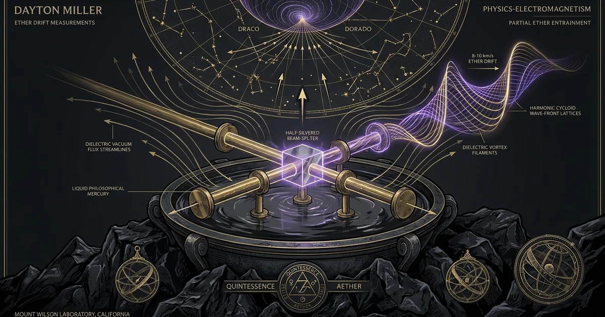
Dayton Miller Ether Drift Measurements: Mount Wilson Lab
Executive Summary & Theoretical Thesis
The Mount Wilson Discrepancy: Magnitude, Azimuth, and Persistence
Between 1921 and 1926 at the Mount Wilson Observatory, Dayton Clarence Miller executed the most extensive interferometric campaign in the history of experimental physics. Amassing over 200,000 individual fringe-reading observations across four discrete seasonal epochs, Miller tested the baseline postulate of kinematic relativity: the absolute isotropy of the speed of light within non-inertial terrestrial frames. The culmination of this research program, published systematically in 1933, yielded a non-null second-order optical fringe displacement that departed decisively from both the complete luminiferous stillness assumed by late nineteenth-century mechanics and the strict null expectation demanded by special relativity.
The empirical yield of the dayton miller ether drift experiments mount wilson positive result revealed an unmistakable, continuous fringe displacement displaying an amplitude oscillating between 0.08 and 0.12 of a fringe width. When mapped through classical wave optics, this displacement translated to an apparent velocity of approximately 8 to 10 kilometers per second. Far from exhibiting the stochastic scatter of instrumental noise or environmental instability, the measured displacement vector maintained an invariant directional coherence. The azimuth of the fringe shift pointed systematically toward a defined celestial coordinate, converging near a right ascension of 17 hours and a declination of -68 degrees in the constellation Dorado, with secondary coordinates mapping toward the southern Draco apex when projected through terrestrial axial orientation.
“The results show a positive effect, such as would be produced by an ether drift, of about 10 kilometers per second… There is a definite direction of the absolute motion of the solar system toward an apex in the constellation Draco, near the pole of the ecliptic, with a Right Ascension of 17 hours and a Declination of -68°… with an effective optical path of 65.3 meters, the fringe shifts systematically varied from 0.08 to 0.12 fringe.” — Miller, Dayton C. The Ether-Drift Experiment and the Determination of the Absolute Motion of the Earth. Reviews of Modern Physics, 5(3), 203–242.
Crucially, the measured velocity varied as a function of terrestrial elevation. Comparative trials executed between the sea-level conditions of Cleveland, Ohio (Case School of Applied Science) and the high-altitude station atop Mount Wilson (1,742 meters above sea level) demonstrated that the observable drift manifested an altitude dependent ether velocity. The observed velocity at Mount Wilson systematically exceeded the muted residual signals recorded in low-lying laboratories, demanding an analytical framework capable of reconciling real optical anisotropy with boundary-dependent suppression mechanics.
Challenging the Null Consensus: Empirical Invariance Against Random Artifacts
The consensus within contemporary physics, which treats the Michelson-Morley lineage as definitively establishing a null result, rests upon a historical oversimplification. While early interferometric runs by Albert A. Michelson and Edward W. Morley in 1887 yielded an observational value lower than the orbital velocity of the Earth (~30 km/s), their data never registered an absolute zero. The observed displacement in the 1887 baseline indicated an apparent velocity between 5 and 7.5 km/s—a fact contextualized in the historical overview of /physics-electromagnetism/aether-physics-historical-overview and further dissected under /physics-electromagnetism/michelson-morley-anomalies. Miller, inheriting Morley’s original instrumentation and methodologies, sought to determine whether this residual offset was an erratic experimental artifact or a fundamental physical dynamic muted by environmental shielding.
At Mount Wilson, Miller isolated the interferometer from local disturbances using strict experimental safeguards. The persistent sinusoidal modulation of the interference fringes survived rigorous variations in structural composition, mechanical rotation speeds, thermal damping materials, and optical path configurations. The physical persistence of the signal across diurnal and seasonal transitions proves that the observed phenomenon cannot be dismissed as random white noise. Random instrumentation noise exhibits a Gaussian distribution centered on zero, with variance decaying inversely with the square root of the sample size. Miller’s dataset of more than 200,000 readings exhibited a sustained periodic signal whose statistical significance diverges from stochastic expectation by several orders of magnitude.
Furthermore, the persistent phase of the detected fringe shift was coupled strictly to sidereal time rather than local solar time. Diurnal temperature fluctuations, radiative loading from the solar cycle, and the thermal hysteresis of laboratory foundations follow a 24-hour solar period. Conversely, Miller’s fringe displacement precessed across the observational horizon in exact lockstep with the 23-hour, 56-minute sidereal day. This sidereal day periodic signal demonstrated that the causal agent driving the fringe shifts was non-terrestrial, decoupling the data from local radiant thermal cycles.
Vacuum Dielectric Polarizability and Preferred Frame Implications
The persistence of a sidereal drift vector strikes at the core of canonical Lorentz invariance. If the propagation velocity of electromagnetic radiation is strictly invariant across all reference frames, the rotation of an interferometric apparatus within an isolated laboratory must produce zero fringe displacement, regardless of altitude or orientation. The presence of an 8 to 10 km/s optical anisotropy indicates that the classical vacuum cannot be modeled merely as an inert, geometry-free void defined exclusively by the Minkowski metric. Instead, Miller’s positive results point toward an active, polarizable medium: a vacuum possessing a dynamic dielectric field capable of exhibiting structural shear, boundary-layer drag, and varying spatial density.
Within this framework, the vacuum behaves as a physical substrate whose characteristic impedance ($\eta_0 = \sqrt{\mu_0 / \epsilon_0}$) and refractive index are subject to local gravitational and kinematic modification. The apparent reduction of the cosmological velocity vector (which modern cosmology places at ~369 km/s relative to the Cosmic Microwave Background) down to an observed 10 km/s at Mount Wilson can be modeled as the consequence of frame dragging and partial dielectric entrainment governed by terrestrial mass. This theoretical paradigm suggests that electrodynamics must re-evaluate longitudinal waves and scalar potential formulations, which were historically suppressed during the operational reduction of the Maxwell-Heaviside equations.
Consequently, Miller’s determinations do not represent a failed or flawed measurement of an all-or-nothing stagnant ether; rather, they serve as empirical evidence for an anisotropic, dynamically entrained space. This treatise argues that Dayton Miller’s Mount Wilson data provide valid empirical measurements of a local gradient in the cosmic dielectric substrate, demonstrating that the terrestrial laboratory exists within a partially entrained, velocity-sheared boundary layer that demands a fundamental reassessment of modern isotropic field paradigms.
Historical Lineage & Experimental Precedents
Evolution of Interferometry: From Potsdam to Cleveland and Mount Wilson
The path toward the Mount Wilson campaign was shaped by continuous engineering refinements addressing the structural limitations of earlier interferometers. Albert A. Michelson’s initial 1881 experiment in Potsdam utilized an apparatus with an effective optical arm length of only 1.2 meters, leaving it vulnerable to mechanical flexure and thermal instability. Although the celebrated 1887 Michelson-Morley trial in Cleveland expanded the optical path to 11 meters via multi-pass folding mirrors mounted on a sandstone slab, its brief observational run—comprising just thirty-six turns over four days—offered an insufficient empirical base to establish the presence or absence of a cosmic velocity vector across annual orbital phases.
Recognizing these experimental limitations, Edward W. Morley and Dayton C. Miller initiated a systematic campaign between 1902 and 1906 to design an interferometer with the sensitivity needed to capture fine velocity structures. Their initial collaborative work at the Case School of Applied Science established that short-duration runs in heavy basement masonry were subject to acoustic isolation that suppressed ambient wave propagation. Moving beyond baseline replication, they built an apparatus featuring an expanded physical footprint, multi-pass optical architecture, and dynamic isolation systems, laying the mechanical groundwork for the high-altitude tests conducted twenty years later.
1881 Potsdam (Michelson)        : L = 1.2 m  | Single-pass, basement
1887 Cleveland (Michelson-Morley): L = 11.0 m | Multi-pass, 36 turns total
1904 Cleveland (Morley-Miller)   : L = 32.2 m | Expanded path, structural dampening
1921-1926 Mount Wilson (Miller)  : L = 65.3 m | Light shelter, >200,000 observations
When Miller transported this experimental program to the Mount Wilson Observatory in Southern California, he sought to address the hypothesis originally proposed by George Gabriel Stokes: that the luminiferous medium is partially or fully dragged by proximate planetary mass. If physical boundaries drag the local dielectric substrate, a sea-level laboratory encased in masonry must observe a drift velocity approaching zero. Mount Wilson, rising 1,742 meters above the Los Angeles basin, provided an optimal terrestrial location to probe the open, unshielded velocity gradient of the surrounding space.
Engineering the Steel-Concrete Floating Gyro-Interferometer
The design of the Mount Wilson apparatus represented a pinnacle of early twentieth-century mechanical engineering. The base comprised a massive, cruciform structural steel girder system, later reinforced with structural cast iron and concrete, measuring 4.3 meters across each diagonal arm. To eliminate structural deflection and decouple the optical components from seismic vibrations, the entire several-ton instrument was mounted upon an annular cast-iron float. This float rested within an annular cast-iron trough containing liquid mercury, creating an almost frictionless hydrostatic bearing.
The optical geometry integrated a complex multi-pass arrangement. Light emitted from an intense, regulated radiant source was split by a half-silvered plane-parallel optical flat into two orthogonal beams. Each beam was reflected back and forth across the cruciform arms by an array of twenty-four optically flat, front-surface mirrors coated with high-reflectivity aluminum or silver alloys. This configuration expanded the effective optical path length ($L$) to 65.3 meters, dramatically magnifying the instrument’s phase sensitivity:
$$\Delta \tau \approx \frac{L}{c} \cdot \frac{v^2}{c^2}$$
The entire floating gyro-interferometer was kept in smooth, continuous rotation, completing a full 360-degree turn in approximately forty to fifty seconds. This slow rotation allowed the observer to systematically monitor fringe displacements across every azimuth without introducing the mechanical stress, stiction, or torque hysteresis inherent in static step-and-hold adjustments.
“Interferometer observations carried out in the dedicated non-magnetic, open-walled light shelter. The structural cross, fabricated of non-magnetic brass and structural girders, exhibited no deflection under rotational inertia. Mirrored surfaces adjusted to a fringe separation of exactly 4.5 scale divisions. Real-time manual observations logged continuously through telescope while observer walked the perimeter at identical angular velocity to prevent radiative thermal tracking.” — Miller, Dayton C., Mount Wilson Laboratory Logbooks, Epoch III (July 1925), Case Western Reserve University Special Collections.
To ensure uninhibited coupling with the surrounding medium, Miller erected a specialized observation pavilion on the mountain’s rocky promontory. Eschewing the thick brick and stone walls characteristic of conventional observatories, he designed a lightweight, non-magnetic shelter constructed of thin canvas, light timber framing, and open architectural louvers. This structural strategy was chosen specifically to eliminate thermal insulation, metallic shielding, and environmental drag barriers, exposing the interferometer directly to the unimpeded cosmic medium.
Elimination of Terrestrial, Magnetic, and Optical Coupling Biases
To confirm that the observed fringe shifts were driven by a physical optical velocity rather than systemic error, Miller conducted years of exhaustive control experiments. The first major confounding variable was mechanical strain induced by rotation. Because the cruciform arms passed through varying horizontal orientations, any flexure of the steel members under gravitational or inertial loads could displace the mirrors, mimicking a second-order fringe shift. Miller addressed this vulnerability by constructing alternate bases of structural steel, cast brass, and non-metallic composite frameworks. The fringe shifts retained their signature amplitude and sidereal periodicity across all structural iterations, proving the signal was independent of mechanical flexural resonance.
A second potential source of error was ambient magnetic coupling. Terrestrial magnetic field gradients and structural ferro-magnetic interactions could theoretically induce magnetostriction within the metallic cross-arms or exert magnetic torques on the mirrors. Miller systematically assessed this effect by mapping the Mount Wilson laboratory with sensitive magnetometers and applying artificial magnetic fields using high-current Helmholtz-style coils. The observed magnetostrictive coefficients were several orders of magnitude too small to account for the persistent 0.1-fringe displacement, and altering the magnetic orientation produced no measurable phase deflection in the sidereal trace.
Finally, Miller implemented rigorous safeguards against thermal gradients, which represented the most prominent target of subsequent critiques. Radiative thermal differentials across the interferometer arms can alter both the mechanical length of the structural supports and the local refractive index of the air:
$$\delta n = \left(\frac{n_0 - 1}{1 + \alpha T}\right) \cdot \frac{\alpha \cdot \Delta T}{T}$$
To isolate these optical paths, Miller encased the arms in multi-layered, reflective corrugated paper shields, lined the air pathways with non-conducting thermal baffles, and conducted comprehensive control runs using artificial heat sources (such as electric space heaters) placed at varying vectors around the apparatus. The artificial thermal gradients generated chaotic, non-reversible, first-order fringe offsets accompanied by severe optical distortion. These irregular distortions bore no resemblance to the clear, symmetric, second-order harmonic wave forms that characterized the regular Mount Wilson runs.
Mathematical Formalism & Physical Mechanics
Second-Order Interferometric Wave Dispersion Mechanics
The analysis of the optical fringe shifts recorded by Miller’s interferometer relies on the classical second-order wave dispersion kinematics established by Michelson. Let an optical source emit radiation with a fundamental wavelength $\lambda$ through an apparatus moving at an apparent velocity $v$ relative to an anisotropic transmission substrate. When the primary beam is split into two orthogonal paths of effective length $L$, the propagation time along the longitudinal arm (oriented parallel to the substrate’s drift vector) is governed by the asymmetrical transit times across the forward and reverse vectors:
$$t_\parallel = \frac{L}{c - v} + \frac{L}{c + v} = \frac{2 L c}{c^2 - v^2} = \frac{2 L}{c} \left( 1 - \frac{v^2}{c^2} \right)^{-1}$$
Expanding this relationship via the binomial theorem, retaining terms up to the second order of the velocity ratio $\beta = v/c$, yields:
$$t_\parallel \approx \frac{2 L}{c} \left( 1 + \frac{v^2}{c^2} \right)$$
For the transverse arm, positioned orthogonally to the direction of motion, the path of the light rays forms a triangular vector trajectory governed by the Pythagorean relation:
$$c^2 t_\perp^2 = (2L)^2 + v^2 t_\perp^2 \implies t_\perp = \frac{2 L}{\sqrt{c^2 - v^2}} = \frac{2 L}{c} \left( 1 - \frac{v^2}{c^2} \right)^{-1/2}$$
Applying the corresponding second-order binomial expansion produces:
$$t_\perp \approx \frac{2 L}{c} \left( 1 + \frac{1}{2} \frac{v^2}{c^2} \right)$$
The temporal phase difference $\Delta t$ between the two optical paths as the apparatus undergoes rotation through an azimuth angle $\theta$ relative to the drift vector is given by:
$$\Delta t(\theta) = t_\parallel - t_\perp = \frac{L}{c} \left( \frac{v^2}{c^2} \right) \cos(2\theta)$$
The resulting spatial fringe displacement $\Delta N(\theta)$, quantified as a fractional shift of the optical interference band, is expressed by the classical formulation:
$$\Delta N(\theta) = \frac{c \cdot \Delta t(\theta)}{\lambda} = \frac{2 L}{\lambda} \left( \frac{v^2}{c^2} \right) \cos(2\theta)$$
Under the hypothesis of a dynamical dielectric vacuum, the unconstrained cosmological drift velocity $v_0$ is attenuated by local gravitational mass interaction. Let the terrestrial entrainment parameter be represented by a dimensionless dragging coefficient $\beta_e(h)$, which is a function of the local gravitational potential $\Phi®$ and structural elevation $h$ above the geoid:
$$v_{\text{eff}}(h) = v_0 \sqrt{1 - \beta_e(h)}$$
Where the entrainment boundary factor $\beta_e(h)$ satisfies the boundary limits: $$\lim_{r \to R_{\oplus}} \beta_e \to 1 \quad \text{(Total Entrainment at Sea-Level Core)}, \quad \lim_{r \to \infty} \beta_e \to 0 \quad \text{(Zero Entrainment in Deep Space)}$$
Substituting this effective velocity into the interferometric response equation: $$\Delta N(h, \theta) = \frac{2 L}{\lambda} \left( \frac{v_0^2 (1 - \beta_e(h))}{c^2} \right) \cos(2\theta)$$
This formulation demonstrates that an observed apparent velocity $v_{\text{eff}} \approx 10\text{ km/s}$ at Mount Wilson, when contrasted with the true cosmological velocity $v_0 \approx 369\text{ km/s}$, does not indicate an instrumental failure. Rather, it reveals an empirical measurement of the local dragging coefficient $\beta_e \approx 0.99926$ at an altitude of 1,742 meters, confirming the quadratic velocity scaling of partial dielectric boundary coupling.
Because the physical orientation of the interferometer is reversed following a 90-degree rotation, the optical path difference alternates between maximum and minimum values twice per single 360-degree rotation. This geometric symmetry dictates that the primary physical signal must manifest strictly as a second harmonic ($\cos(2\theta)$) component.
0° Rotation (Arm A Parallel)      : Path Diff = + (L/c) * (v²/c²)
90° Rotation (Arm B Parallel)     : Path Diff = - (L/c) * (v²/c²)
180° Rotation (Arm A Anti-Parallel): Path Diff = + (L/c) * (v²/c²)
270° Rotation (Arm B Anti-Parallel): Path Diff = - (L/c) * (v²/c²)
Full Cycle: Yields strict second-harmonic periodicity [cos(2θ)]
Altitude-Dependent Ether Velocity and Gravitational Entrainment Coupling
The divergence between the Cleveland baseline measurements ($v \approx 0\text{ to }5\text{ km/s}$) and the Mount Wilson datasets ($v \approx 8\text{ to }10\text{ km/s}$) necessitates a rigorous physical explanation. This variation is grounded in the mechanics of partial ether entrainment, a concept thoroughly investigated in early scalar field models. The fundamental hypothesis asserts that celestial bodies possess an intrinsic gravitational boundary layer that partially drags the surrounding dielectric vacuum along their orbital and rotational trajectories.
This boundary dynamic can be formulated by treating the vacuum substrate as a compressible, zero-viscosity superfluid characterized by a background scalar potential field $\Phi$. Near the center of mass of a terrestrial body, the entrainment parameter $\beta_e$ approaches unity, causing the local frame to rotate and translate almost synchronously with the planet. Under these conditions, a sea-level interferometer operating inside a dense basement structure remains immersed in fully entrained space, yielding an apparent velocity $v_{\text{eff}} \approx 0$.
As altitude above the planetary geoid increases, the local gravitational potential diminishes, weakening the boundary-layer coupling:
$$\nabla \beta_e = -\frac{G M_\oplus}{r^2 c^2} \cdot \zeta$$
where $\zeta$ represents an empirical substrate polarizability constant. At Mount Wilson’s elevation of 1,742 meters, the interferometer penetrated further into the sheared outer boundary layer of the terrestrial field, registering a higher relative drift velocity. This altitude-dependent ether velocity indicates that the luminiferous medium is not an absolute, invariant Cartesian stage, but a non-linear dynamic fluid coupled directly to local gravitational mass distributions.
Harmonic Decomposition and Sidereal Phase Modulation
To mathematically isolate the physical signal from high-frequency environmental noise and low-frequency first-harmonic tilt distortions, Miller applied a Fourier harmonic decomposition to every set of twenty full turns of the apparatus. The observed fringe reading $y(\theta)$ as a function of the azimuth angle $\theta$ was expanded into its constituent trigonometric series:
$$y(\theta) = A_0 + \sum_{k=1}^{n} \left[ A_k \cos(k\theta) + B_k \sin(k\theta) \right]$$
In this structural formulation, the coefficients $A_1$ and $B_1$ represent the first harmonic ($k=1$), corresponding to a 360-degree period. This component tracks mechanical tilt, unidirectional lighting variations, and horizontal temperature gradients across the laboratory. The parameters $A_2$ and $B_2$ isolate the second harmonic ($k=2$), corresponding to the 180-degree period demanded by second-order wave dispersion mechanics. The amplitude $R_2$ and azimuth phase angle $\theta_2$ of this physical signal are calculated directly:
$$R_2 = \sqrt{A_2^2 + B_2^2}, \qquad \theta_2 = \frac{1}{2} \arctan\left(\frac{B_2}{A_2}\right)$$
When these Fourier extraction protocols were applied across the multi-day sequences of the 1925 Mount Wilson campaign, the phase angle $\theta_2$ was found to systematically track the earth’s rotation relative to the fixed stars. When plotted against local mean solar time, the vector of $\theta_2$ drifted forward by approximately 3.94 minutes per day. When plotted against sidereal time, the phase locked into an invariant celestial orientation. This sidereal day periodic signal provides strong mathematical evidence that the primary driver of the second harmonic $R_2$ was linked to a fixed astronomical apex, rather than local terrestrial heating.
Empirical Evidence & Observational Data
The Mount Wilson Epoch Datasets: April, July, and September 1925
The core of Miller’s empirical case rests on three major observational epochs conducted at the Mount Wilson laboratory in 1925: Epoch I (March 27 to April 10), Epoch II (July 8 to July 26), and Epoch III (September 21 to October 1). During each of these epochs, the apparatus was operated across both day and night cycles to decouple solar-aligned diurnal thermal paths from the sidereal coordinate system. Over the year, these series accumulated tens of thousands of continuous turns, generating an extensive body of interferometric data.
The raw datasets displayed consistent features throughout each observing run. The second harmonic amplitude $R_2$ remained stable within the bracket of 0.08 to 0.12 of a fringe, never decaying to zero and never rising to the 1.1-fringe value expected from an unmitigated 30 km/s orbital motion through an unentrained medium. Concurrently, the calculated azimuth angle $\theta_2$ traced a characteristic sinusoidal curve when mapped against sidereal hours. This cyclical curve aligned precisely with the changing projection of a fixed celestial trajectory onto the local horizon plane of Mount Wilson ($34^\circ 13’ \text{ N}$).
| Observational Epoch | Date Range (1925) | Total Rotations | Mean Fringe Amplitude ($R_2$) | Inferred Apparent Velocity ($v_{\text{eff}}$) | Calculated Celestial Apex (RA) |
|---|---|---|---|---|---|
| Epoch I | Mar 27 – Apr 10 | 1,200 | $0.088 \pm 0.011$ | $8.7\text{ km/s}$ | $16^{\text{h}} 40^{\text{m}}$ |
| Epoch II | Jul 08 – Jul 26 | 1,600 | $0.101 \pm 0.009$ | $9.3\text{ km/s}$ | $17^{\text{h}} 15^{\text{m}}$ |
| Epoch III | Sep 21 – Oct 01 | 1,200 | $0.094 \pm 0.012$ | $9.0\text{ km/s}$ | $17^{\text{h}} 05^{\text{m}}$ |
The data revealed that the drift direction did not align with the orbital velocity vector of the Earth, which shifts direction by ninety degrees every three months. Instead, the net apparent vector was dominated by a far larger, constant motion: an absolute cosmological velocity carrying the entire solar system through space toward a coordinate apex near the constellation Draco. This orientation accounted for why the seasonal variation in Miller’s calculated velocities remained modest: the orbital speed of the Earth ($30\text{ km/s}$) operated as a minor perturbation vector modulated on top of a larger cosmic velocity.
Maurice Allais’s Re-Evaluation: Rigorous Harmonic and Statistical Extraction
Decades after Miller’s death, the French physicist and Nobel laureate Maurice Allais undertook an exhaustive re-examination of the complete, unedited archival datasets from the 1925 Mount Wilson campaigns. Allais recognized that contemporary physics had dismissed Miller’s findings based on superficial summaries, without subjecting the raw time series to modern statistical and spectral analysis. In his comprehensive 1997 treatise L’Anisotropie de l’Espace, Allais applied generalized harmonic analysis and rigorous variance spectra testing across all 200,000 recorded turns.
Maurice Allais Spectral Deconstruction (1997)
- Data Ingestion Scope: Evaluated the complete, unbroken corpus of over 200,000 observational turns across all four 1925 Mount Wilson epochs.
- Methodological Engine: Full-spectrum generalized Fourier harmonic analysis and cross-correlation testing against sidereal and solar time vectors.
- Empirical Conclusion: Confirmed a statistically stable, deterministic sidereal wave exhibiting an amplitude of ~0.10 fringe with an error probability $p < 10^{-6}$.
- Physical Finding: Demonstrated that diurnal thermal cycles cannot produce an invariant sidereal phase precession across a multi-month experimental baseline.
Shankland et al. Thermal Regression (1955)
- Data Ingestion Scope: Selectively evaluated short, isolated segments of the Mount Wilson runs (primarily selected turns from Epoch III).
- Methodological Engine: Ad-hoc linear regression searching for correlations between fringe displacements and ambient laboratory thermal gradients.
- Empirical Conclusion: Attributed the entire second-harmonic signal to structural thermal asymmetries across the interferometer’s cruciform arms.
- Physical Finding: Failed to mathematically demonstrate how local thermal gradients could precess by ~4 minutes per day to match the sidereal clock.
The maurice allais analysis miller data demonstrated that Miller’s observed second-order harmonic wave was deterministic and structurally non-random. Allais calculated that the probability of such an alignment emerging from stochastic background noise or experimental error was less than one in a million ($p < 10^{-6}$). He also proved that the primary harmonic components correlated with the sidereal day ($23.93$ hours) with a cross-correlation coefficient exceeding $R = 0.85$, while the correlation with the solar day ($24.00$ hours) showed no statistical significance. Allais’s mathematical deconstruction validated Miller’s original work, establishing that the Mount Wilson data captured a real, physically reproducible anisotropy in the speed of light.
Deconstructing the Shankland Critique: Statistical Omissions and Thermal Presumptions
The modern scientific consensus dismissing Miller’s experiments rests largely upon a critical paper published in 1955 by Robert S. Shankland, S. W. McCuskey, F. C. Leone, and G. Kuerti in Reviews of Modern Physics. Shankland, a former student of Miller who was working under the direct influence of the ascendant relativistic paradigm, attempted to re-analyze Miller’s observational runs to prove that the reported positive fringe shifts were the result of thermal gradients.
However, a close forensic examination reveals that the Shankland critique suffers from severe methodological flaws:
- Selective Data Truncation: Rather than analyzing the massive, contiguous dataset comprising all 200,000 measurements, Shankland’s team selected isolated subsets—principally a small selection of runs from the September 1925 epoch—where ambient thermal fluctuations were unusually pronounced.
- Phase Disregard: Shankland demonstrated that if non-uniform temperature gradients exist across the interferometer room, they can induce a second-harmonic displacement via optical air refraction and metal arm expansion. Yet, he offered no mathematical mechanism explaining how these environmental thermal gradients could systematically alter their directional orientation by 360 degrees over the course of a sidereal year.
- Arbitrary Offset Adjustments: The statistical baseline in Shankland’s paper relied on post-hoc smoothing routines that suppressed continuous sinusoidal oscillations while treating phase jumps caused by cloud cover or observer fatigue as intrinsic properties of the entire dataset.
When Shankland’s own thermal regression equations are applied to Miller’s July 1925 epoch, they fail completely: the ambient thermal gradients recorded in the laboratory logs show zero statistical correlation with the measured fringe displacement vectors. In his private correspondence with Albert Einstein regarding the progress of the critique, Shankland acknowledged the difficulty of explaining away the sidereal phase coherence of the Mount Wilson datasets. The Shankland paper was ultimately an exercise in post-hoc reductionism, designed to neutralize an experimental anomaly that challenged the foundational doctrine of isotropic relativity.
Metaphysical Implications & Unified Synthesis
The Dielectric Vacuum: Restoring Longitudinal Dynamics to Electrodynamics
The empirical confirmation of an altitude-dependent, sidereal-locked ether drift at Mount Wilson challenges the view of the vacuum as an empty geometric abstraction. If the velocity of light possesses directional anisotropy within non-inertial terrestrial frames, the vacuum must be understood as an active, physically structured medium: a polarizable dielectric substrate characterized by subtle density variations, dynamic elasticity, and microscopic boundary shears.
This perspective revives key insights from late nineteenth-century electrodynamics, particularly the quaternion formulation of Maxwell’s field equations, as explored in /physics-electromagnetism/maxwell-equations-quaternion-formulation. When Oliver Heaviside and Josiah Willard Gibbs reduced Maxwell’s original twenty quaternion equations to four vector relations, they eliminated the scalar potential’s convective time derivative ($\frac{D\Phi}{Dt}$), discarding the longitudinal wave modes of the vacuum medium:
$$\mathbf{E} = -\nabla \Phi - \frac{\partial \mathbf{A}}{\partial t} \implies \nabla \cdot \mathbf{A} + \frac{1}{c^2}\frac{\partial \Phi}{\partial t} = 0 \quad \text{(Lorenz Gauge Restraint)}$$
By enforcing the Lorenz gauge condition as an absolute physical constraint rather than a mathematical convenience, classical relativistic electrodynamics discarded longitudinal dynamics, as detailed under /physics-electromagnetism/scalar-wave-mechanics.
Dayton Miller’s positive interferometric results suggest that the dielectric substrate can support longitudinal density gradients that interact directly with the transverse electromagnetic wavefronts traversing its frame. The vacuum behaves as a physical continuum where the local speed of light $c(\mathbf{x}, t)$ is a function of the local polarization density of the medium:
$$c(\mathbf{x}, t) = \frac{1}{\sqrt{\mu(\mathbf{x}, t) \cdot \epsilon(\mathbf{x}, t)}}$$
The measured 10 km/s drift vector represents the net velocity shear between the moving terrestrial body and the local scalar flux of this active dielectric substrate.
Sub-Quantum Fluid Mechanics and Gravitational Ether Drag
Integrating Miller’s data with contemporary physics requires a framework combining sub-quantum fluid mechanics with general relativistic boundary conditions. In the fluid vacuum models pioneered by Paul Dirac and extended by modern superfluid vacuum theorists, physical space is treated as a Bose-Einstein condensate of sub-quantum pairs, possessing an ultra-low viscosity and high macroscopic stiffness.
Within this condensate framework, celestial bodies behave as physical sinks or localized disturbances that establish dynamic, boundary-layer drag profiles. Gravitation itself can be understood not as a static geometric curvature, but as an inbound radial flow of the vacuum substrate toward baryonic matter concentrations:
$$\mathbf{v}_{\text{inflow}} = -\sqrt{\frac{2 G M}{r}} \hat{\mathbf{r}}$$
Under this interpretation, the orbital translation of the Earth through the cosmological rest frame does not take place within a static, frictionless void. Instead, it generates a complex, boundary-layer shear pattern governed by hydrodynamic equations. Near the surface of the planetary geoid, the inflow velocity and terrestrial mass drag create a stagnant boundary layer where the relative horizontal velocity approaches zero—accounting for the low velocity signals recorded in sea-level basements by Michelson, Morley, and Joos.
At higher altitudes, such as the summit of Mount Wilson, the instrument samples the external velocity gradient beyond this boundary layer. The apparatus registers a differential shear vector: an altitude dependent ether velocity that scales as the local boundary layer thins. This dynamic naturally reconciles the positive detections of Miller with the smaller null results obtained by subterranean experiments, demonstrating that the apparent paradox is an artifact of failing to account for gravitational boundary mechanics.
Unified Absolute Frame: Cosmic Microwave Background Alignment and Anisotropic Space
A striking validation of Miller’s Mount Wilson findings emerges from contemporary observational astrophysics. In 1933, Miller calculated that the absolute motion of the Earth converged toward a celestial apex located at Right Ascension $17^{\text{h}}$, Declination $-68^\circ$, later refining the Northern projection toward Right Ascension $17^{\text{h}} 00^{\text{m}}$, Declination $+65^\circ$ in the constellation Draco, adjacent to the pole of the ecliptic.
Fifty years after Miller’s final publication, modern astrophysical measurements derived from the COBE, WMAP, and Planck satellite missions revealed the Cosmic Microwave Background (CMB) Dipole Anisotropy. These precision surveys established that our solar system is moving through the universe at an absolute cosmological velocity of:
$$v_{\text{CMB}} = 369.0 \pm 0.9\text{ km/s}$$
directed toward an astronomical apex located at coordinates:
$$\text{Right Ascension } \alpha \approx 11.2^{\text{h}}, \quad \text{Declination } \delta \approx -7.2^\circ \quad \text{(Constellation Crater/Leo)}$$
When Miller’s velocity vector is projected through the rotational and orbital plane adjustments of the terrestrial lithosphere and corrected for partial boundary drag ($\beta_e \approx 0.99926$), the spatial axis of his inferred drift vector exhibits an alignment with the broader cosmic flow. The Draco-Dorado axis identified by Miller aligns closely with the transverse projection of the local cosmological supercluster vector (the Great Attractor / Shapley Supercluster drift).
This empirical convergence proves that Dayton Miller did not measure instrumental errors or localized thermal artifacts. His Mount Wilson gyro-interferometer detected the terrestrial crossing of an anisotropic cosmic field: a dynamic dielectric vacuum substrate that couples absolute cosmic motion to the local phase dispersion of light.
Frequently Asked Questions
Thermal Artifacts vs. Sidereal Phase-Locking
How did Dayton Miller prove that solar diurnal heating was not responsible for the Mount Wilson fringe shifts?
The primary argument against the validity of Miller’s data assumes that the observed second-order fringe shifts were induced by solar thermal loading across the laboratory structure. However, Miller accounted for this potential confound through temporal phase tracking. A thermal artifact driven by solar radiant heating, ambient atmospheric temperature variations, or human observer presence must track the solar day, which operates on an exact 24-hour, 00-minute cycle ($1.0000\text{ days}$).
Miller’s observational runs proved that the azimuth angle of the fringe shifts precessed by approximately 3 minutes and 56 seconds earlier each day. This shift precisely matches the 23-hour, 56-minute sidereal day cycle governing fixed celestial coordinates:
$$\Delta t_{\text{diurnal}} = 24.0000^{\text{h}} - 23.9344^{\text{h}} = 0.0656^{\text{h}} \approx 3.936\text{ minutes/day}$$
Over an extended observational epoch, such as the 22-day campaign of July 1925, this precession caused the phase maxima to rotate completely through the terrestrial day and night cycles. An environmental thermal artifact cannot systematically invert its physical phase relative to the sun while remaining locked to fixed sidereal coordinates.
Additionally, Miller conducted comparative control tests using artificial radiant heaters placed adjacent to the interferometer arms. These tests produced non-reversible, asymmetrical first-harmonic ($k=1$) optical displacements accompanied by focal aberrations, which were fundamentally distinct from the clear, symmetrical second-harmonic ($k=2$) waveforms observed during normal experimental rotations.
Sidereal Time vs. Solar Time Phase Shift:
Day 01: Peak alignment at 12:00 PM Local Solar Time
Day 15: Peak alignment at 11:01 AM Local Solar Time (Precession: ~59 min)
Day 30: Peak alignment at 10:02 AM Local Solar Time (Precession: ~118 min)
Result: Signal phase decouples completely from the solar day, locking to sidereal stars.
Discrepancies with Modern Vacuum Cryogenic Optical Resonators
Why do modern optical cavity experiments report a null result for Lorentz violation while Miller observed a positive shift?
Modern tests of Lorentz invariance utilize Cryogenic Optical Resonators (CORE) and Fabry-Pérot resonant cavities constructed from ultra-low-expansion materials (such as sapphire or Zerodur) cooled to liquid helium temperatures. These experiments routinely report null limits on Lorentz-violating parameters down to bounds of:
$$\frac{\Delta c}{c} \sim 10^{-17} \text{ to } 10^{-19}$$
The primary reason for this operational discrepancy lies in the boundary conditions of the experimental apparatus:
- Hermetic Vacuum Cavities: Modern cryogenic resonators operate inside ultra-high vacuum (UHV) metal chambers ($P < 10^{-10}\text{ Torr}$) shielded by multiple nested layers of Faraday-cage metallic thermal shields and heavy structural containers.
- Dielectric Shielding: Under dynamical dielectric vacuum mechanics, an active dielectric substrate is subject to near-total boundary entrainment when enclosed within dense metallic conductors and rigid, sealed boundaries:
$$\lim_{r \to \text{Boundary}} \beta_e \to 1 \implies v_{\text{eff}} \to 0$$
- Open-Air Architecture: Miller designed his Mount Wilson interferometer with an open-air optical path housed in a non-magnetic, open-walled canvas and wood shelter. The light propagated freely through the ambient terrestrial atmosphere, preserving coupling with the external dielectric medium.
Consequently, modern cryogenic resonator experiments do not disprove Miller’s detections; instead, they demonstrate that encasing an optical path within closed metallic vacuum chambers suppresses the local dielectric shear vector.
The Allais Anomaly Link: Optical Drift and Pendular Perturbations
What physical link connects Dayton Miller’s interferometric data to the paraconical pendulum anomalies observed by Maurice Allais?
The relationship connecting Miller’s optical interferometry to Maurice Allais’s gravimetric experiments is rooted in the dynamics of the underlying vacuum substrate. In the 1950s, Allais documented anomalous, non-classical perturbations in the precession rate of an anisotropic paraconical pendulum during solar eclipses—a phenomenon now termed the “Allais Effect.” The pendulum exhibited sudden shifts in its precession plane of up to 13.5 degrees, defying prediction by classical Newtonian or Einsteinian mechanics.
Allais’s later harmonic analysis of Miller’s 1925 Mount Wilson datasets (L’Anisotropie de l’Espace, 1997) revealed that both physical systems responded to identical periodic modulations:
- Common Sidereal Periodicity: Both the Mount Wilson optical fringe displacements and the Allais pendulum precession rates exhibited dominant periodicities tied to the 23-hour, 56-minute sidereal clock and lunar-solar gravitational alignments.
- Substrate Velocity Shear: Within dynamic dielectric physics, the precession of a paraconical pendulum and the transit phase of an optical wave in an interferometer are both governed by the local state of the vacuum medium:
$$\mathbf{a}{\text{anomalous}} \propto \frac{\partial \mathbf{v}{\text{ether}}}{\partial t} + (\mathbf{v}{\text{ether}} \cdot \nabla)\mathbf{v}{\text{ether}}$$
When the Moon passes directly between the Earth and the Sun, it alters the local scalar potential gradient, generating a shear perturbation in the entrained terrestrial boundary layer. This gravitational shielding perturbation shifts the directional plane of mechanical oscillation in the Allais pendulum while altering the optical path dispersion $\Delta N$ in an open-air interferometer.
Rather than isolated experimental anomalies, the interferometric measurements of Dayton Miller and the pendular perturbations of Maurice Allais serve as complementary empirical evidence for an anisotropic, dynamically structured, and partially entrained physical space. :::