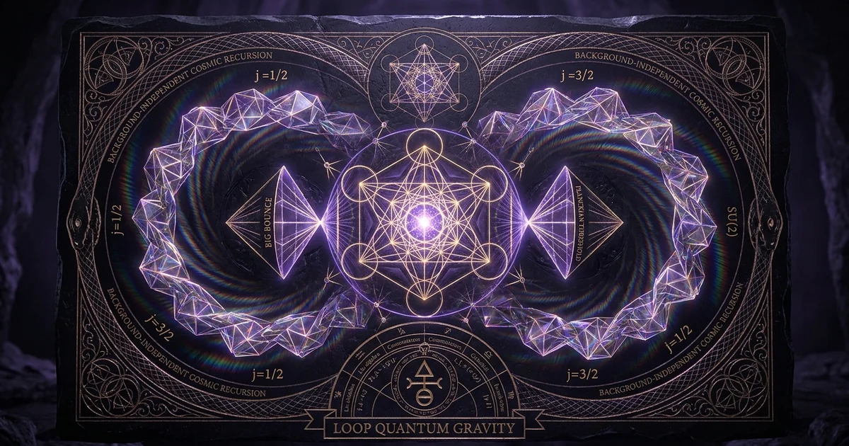
Loop Quantum Gravity: Spin Networks & Discrete Spacetime

Executive Summary & Theoretical Thesis

The Breakdown of Perturbative Quantization

The fundamental crisis of modern theoretical physics resides in the mathematical and conceptual incompatibility between general relativity and perturbative quantum field theory. When conventional quantization protocols are applied to the gravitational field via the split of the metric tensor into a static Minkowski background and a dynamic perturbation, $g_{\mu\nu} = \eta_{\mu\nu} + \kappa h_{\mu\nu}$, the resulting field theory proves to be perturbatively non-renormalizable at two loops without matter, and at one loop in the presence of generic matter couplings. The gravitational coupling constant $G$ possesses negative mass dimension ($[G] = M^{-2}$ in natural units $\hbar = c = 1$), which fundamentally guarantees that loop-momentum expansions generate an infinite tower of ultraviolet divergences requiring an infinite sequence of non-predictive counterterms.

Perturbative quantum gravity assumes that gravitational excitations—traditionally identified as massless, spin-2 gravitons—propagate upon an inert, fixed background stage. This methodological posture fundamentally violates the foundational insight of Einstein’s general theory of relativity: gravity is not a material force propagating through an antecedent geometric vessel, but rather the manifestation of the dynamic geometry of the spacetime manifold itself. By forcing the dynamic field $g_{\mu\nu}$ into the rigid architecture of an unyielding background metric $\eta_{\mu\nu}$, the perturbative framework inadvertently divorces the field from its core property of active diffeomorphism invariance. Consequently, the high-energy trans-Planckian regime induces severe mathematical pathological divergences, indicating that the smooth continuum approximation collapses catastrophically as energy densities approach the Planck scale ($E_P \sim 10^{19}\text{ GeV}$).

Background Independence as an Ontological Axiom

Loop Quantum Gravity (LQG) resolves this fundamental impasse by establishing background independence as its non-negotiable ontological axiom. In this non-perturbative paradigm, there is no pre-existing metric framework, no ambient spatial coordinate system, and no global temporal parameter against which physical processes unfold. Instead, spatial geometry is quantized directly as an autonomous physical entity. Space does not “contain” gravitational fields; dynamic, relational physical states are the geometry. The physical coordinates marking spacetime points possess no intrinsic ontological reality; they are merely gauge parameters subordinated to the group of active four-dimensional diffeomorphisms $\text{Diff}(M)$.

By systematically applying Dirac’s canonical quantization algorithm to constrained Hamiltonian systems, Loop Quantum Gravity constructs a rigorous non-perturbative framework wherein the metric structure is elevated to an operator-valued distribution acting upon a background-independent Hilbert space. The primary consequence of this formulation is that quantum states are defined purely relationally. Points on the spatial manifold obtain physical meaning only through the coincidence of field configurations. The theory replaces the classical differential geometry of smooth pseudo-Riemannian manifolds $(\mathcal{M}, g)$ with a purely algebraic and combinatorial structure, wherein the fundamental fabric of reality is composed of interconnected quanta of spatial geometry governed by non-Abelian gauge groups.

Spatial Quantization and the Demise of the Continuum

The central physical consequence of Loop Quantum Gravity is the absolute structural breakdown of the spatial continuum at the scale of the planck-length ($\ell_P = \sqrt{\frac{\hbar G}{c^3}} \approx 1.616 \times 10^{-35}\text{ m}$). Spacetime is not infinitely divisible. Classical field theories operating over continuous spatial coordinates $\vec{x} \in \mathbb{R}^3$ are revealed to be long-wavelength, thermodynamic approximations—coarse-grained effective field theories that mask an underlying, discrete quantum topology. Physical spatial attributes, specifically geometric area and physical three-dimensional volume, are manifested through self-adjoint quantum operators possessing purely discrete eigenvalue spectra.

The continuum is replaced by an interconnected lattice of relational states where geometric measurements correspond to transitions between fundamental eigenvalues of quantum operators. The transition from continuous spatial metrics to discrete quanta of geometry directly resolves the pathological singularities that historically crippled general relativity. Because spatial metrics cannot collapse below non-zero ground-state eigenvalues proportional to $\ell_P^2$ and $\ell_P^3$, infinite energy densities and point-like spatial collapses are rendered physically non-realizable. Space emerges through the collective macroscopic coherence of these microscopic geometric primitives, establishing a paradigm where geometry is quantized intrinsically from first principles.

Historical Lineage & Experimental Precedents

Penrose Combinatorial Networks and Relational Spin

The conceptual origins of loop quantum gravity trace directly to the combinatorial spacetime program initiated by Roger Penrose in his 1971 treatise Angular Momentum: An Approach to Combinatorial Space-Time. Dissatisfied with the continuum assumptions underpinning both quantum field theory and general relativity, Penrose posited that a genuinely unified quantum theory of spacetime must be constructed from purely discrete, algebraic primitives rather than continuous geometric coordinates. He demonstrated that systems constructed solely from the recoupling algebra of the $SU(2)$ group—the fundamental universal covering group of classical three-dimensional rotations—could generate angular spatial relationships without any reference to an embedding space.

Penrose constructed abstract combinatorial graphs composed of directional lines labeled by non-negative half-integers corresponding to total angular momentum representations $j \in \frac{1}{2}\mathbb{N}$. These lines intersected at vertices structured as three-valent invariant tensors, matching the Wigner $3j$-symbols of quantum angular momentum theory. Penrose’s “Spin Geometry Theorem” proved that as the topological complexity and representation quantum numbers of these abstract relational graphs grew large, they naturally converged to classical three-dimensional directional metrics. The angular separation between discrete units of physical spin matched the classical Euclidean geometric inner product:

$$\cos \theta \sim \frac{\mathbf{J}_1 \cdot \mathbf{J}_2}{|\mathbf{J}_1||\mathbf{J}_2|}$$

Crucially, Penrose’s spin networks did not live in space; they were relational graphs whose combinatorial connections generated the phenomenological appearance of spatial directions from pure group theory, laying the direct mathematical foundation for background-independent quantum geometry.

The Ashtekar Connection Formalism

Despite the philosophical promise of Penrose’s combinatorial program, it remained isolated from the dynamic equations of general relativity for over a decade. Classical canonical general relativity, originally formulated by Arnowitt, Deser, and Misner (ADM) in 1959, decomposed the four-dimensional metric tensor $g_{\mu\nu}$ into an intrinsic 3-metric $q_{ab}$ on a spatial hypersurface $\Sigma$, accompanied by a lapse function $N$, a shift vector $N^a$, and the canonically conjugate momentum field:

$$p^{ab} = \frac{\sqrt{q}}{16\pi G}\left(K^{ab} - q^{ab}K\right)$$

where $K_{ab}$ is the extrinsic curvature. The resulting ADM Hamiltonian constraint:

$$\mathcal{H} = \frac{16\pi G}{\sqrt{q}}\left(p_{ab}p^{ab} - \frac{1}{2}p^2\right) - \frac{\sqrt{q}}{16\pi G}{}^{(3)}R = 0$$

exhibited catastrophic non-polynomial non-linearities in the spatial metric and its derivatives, frustrating non-perturbative canonical quantization efforts via the Wheeler-DeWitt equation.

The breakthrough occurred in 1986, when Abhay Ashtekar introduced a revolutionary change of variables. Drawing upon chiral formulations of the Palatini action, Ashtekar redefined the phase space of general relativity by replacing the spatial metric $q_{ab}$ with an $SU(2)$ connection field $A_a^i(x)$—termed the Ashtekar-Barbero connection—and its canonically conjugate densitized triad flux field $E_i^a(x)$:

$$A_a^i(x) = \Gamma_a^i(x) + \gamma K_a^i(x)$$

$$E_i^a(x) = \frac{1}{2} \epsilon_{ijk} \epsilon^{abc} e_b^j e_c^k = \sqrt{\det q} , e_i^a(x)$$

Here, $e_i^a$ represents the spatial triad (or dreibein) satisfying $q_{ab}e_i^a e_j^b = \delta_{ij}$, $\Gamma_a^i$ denotes the compatible spin connection, $K_a^i = K_{ab}e^{b i}$ encodes the extrinsic curvature, and $\gamma \in \mathbb{R}^+$ is the dimensionless Barbero-Immirzi parameter. This transformation mapped general relativity from a pathological metric-based theory into an $SU(2)$ non-Abelian Yang-Mills gauge theory supplemented by spatial diffeomorphism and scalar constraints. The canonical Poisson bracket between the new conjugate variables assumed an impeccably simple, canonical form:

$${A_a^i(x), E_j^b(y)} = 8\pi G \gamma , \delta_a^b \delta_j^i \delta^3(x - y)$$

This profound shift from metric tensor components to gauge connection variables enabled physicists to import the non-perturbative mathematical apparatus of gauge field theories directly into the quantum mechanics of gravitation.

Wilson Loops and the Rovelli-Smolin Loop Representation

In 1988 and 1990, Carlo Rovelli and Lee Smolin synthesized Ashtekar’s gauge variables with Penrose’s combinatorial concepts by constructing the loop representation of quantum general relativity. Recognizing that point-like evaluations of connection fields $A_a^i(x)$ are unphysical and gauge-dependent, Rovelli and Smolin shifted the fundamental state space to non-local, gauge-invariant non-Abelian Wilson loops. For a closed continuous loop $\alpha: S^1 \to \Sigma$, the Wilson loop functional is defined as the path-ordered exponential trace:

$$W_\alpha[A] = \text{Tr} \left( \mathcal{P} \exp \oint_\alpha A_a^i \tau_i , dx^a \right)$$

where $\tau_i = -\frac{i}{2}\sigma_i$ are the generators of the $\mathfrak{su}(2)$ Lie algebra satisfying $[\tau_i, \tau_j] = \epsilon_{ijk}\tau_k$.

Rovelli and Smolin demonstrated that quantum state functionals $\Psi[A]$ constructed over collections of intersecting Wilson loops spontaneously diagonalized the spatial geometry operators and rigorously satisfied the $SU(2)$ Gauss gauge constraint:

$$G_i = \mathcal{D}a E_i^a = \partial_a E_i^a + \epsilon{ijk} A_a^j E_k^a = 0$$

Furthermore, by reformulating the basis states from isolated loops to intersecting networks of lines labeled by representations of $SU(2)$, they reconstructed Penrose’s spin networks directly within Ashtekar’s phase space. In their landmark 1995 papers, Rovelli and Smolin proved that when spatial area and volume operators are applied to these spin network states, the continuous spectrum predicted by classical differential geometry completely evaporates. Instead, spatial geometry decomposes into a discrete set of quantifiable quantum transitions, providing an exact mathematical realization of spatial discreteness derived systematically from an exact canonical quantization of Einstein’s field equations.

Mathematical Formalism & Physical Mechanics

The Holonomy-Flux Commutation Algebra

The canonical quantization of classical fields requires the construction of non-singular, smeared observables to prevent distributional delta-function divergences at coincidence points. In Loop Quantum Gravity, this smearing protocol is guided by geometric background independence. The connection field $A_a = A_a^i \tau_i$ is naturally a differential 1-form, dictating that it must be integrated along one-dimensional curves $e$ embedded in the spatial manifold $\Sigma$. This operation generates the group-valued holonomy $h_e[A] \in SU(2)$:

$$h_e[A] = \mathcal{P} \exp \left( \int_e A_a^i(x) \tau_i , \frac{dx^a}{ds} , ds \right)$$

Conversely, the conjugate densitized triad $E_i^a$ possesses the transformation properties of a vector density of weight +1, making it dual to a 2-form via the Levi-Civita symbol: $\tilde{E}i = \frac{1}{2}\epsilon{abc} E_i^a dx^b \wedge dx^c$. Consequently, the triad must be smeared over a two-dimensional surface $S \subset \Sigma$, producing the algebra-valued flux $E_i(S)$:

$$E_i(S) = \int_S E_i^a(x) , n_a(x) , d^2\sigma$$

where $n_a(x) = \epsilon_{abc} \frac{\partial x^b}{\partial \sigma^1} \frac{\partial x^c}{\partial \sigma^2}$ is the normal 1-form to the surface parameterization.

The Poisson bracket between a 1D holonomy along path $e$ and a 2D flux across surface $S$ eliminates the spatial Dirac delta distributions, yielding a clean, highly structured quantum operator commutation relation—the holonomy-flux-algebra:

$${h_e[A], E_i(S)} = \begin{cases} \pm 8\pi G \gamma , h_{e_1}[A] , \tau_i , h_{e_2}[A], & e \cap S \neq \emptyset \ 0, & e \cap S = \emptyset \end{cases}$$

Here, the intersection orientation dictates the sign, and $e_1, e_2$ represent the curve segments bifurcated by the crossing of $S$. The holonomy acts as a multiplicative configuration operator, while the flux acts as a Lie-derivative differential momentum operator on the gauge group, establishing the Kinematical representation for quantum geometry. Further technical derivations linking these configurations can be explored through canonical analyses of /physics-electromagnetism/ashtekar-variables-canonical-gravity.

Kinematical Hilbert Space and the Cylindrical Functions

The rigorous mathematical foundation of Loop Quantum Gravity rests upon its Kinematical Hilbert Space $\mathcal{H}_{kin}$, constructed independently of any background metric through the projective limit of spaces of cylindrical functions. Let $\Gamma \subset \Sigma$ be an oriented spatial graph composed of $E$ edges and $V$ vertices. A functional $\Psi[A]$ is cylindrical with respect to $\Gamma$ if its functional dependence on the infinite-dimensional connection space $\mathcal{A}$ factorizes through the holonomies along the finite set of edges of $\Gamma$:

$$\Psi_\Gamma[A] = f(h_{e_1}[A], h_{e_2}[A], \dots, h_{e_E}[A])$$

where $f: SU(2)^E \to \mathbb{C}$ is a smooth function over the compact Lie group manifold.

The space of all cylindrical functions $\text{Cyl}(\mathcal{A})$ over all possible finite graphs is rendered an inner product space through the integration over the Ashtekar-Lewandowski measure $d\mu_{AL}$:

$$\langle \Psi_\Gamma | \Phi_{\Gamma’} \rangle = \int_{\overline{\mathcal{A}}} \overline{\Psi_\Gamma[A]} , \Phi_{\Gamma’}[A] , d\mu_{AL}(A)$$

The Ashtekar-Lewandowski measure leverages the unique, bi-invariant normalized Haar measure $d\mu_H$ available on compact Lie groups:

$$\langle \Psi_\Gamma | \Phi_\Gamma \rangle = \int_{SU(2)^E} \overline{f(g_1, \dots, g_E)} , g(g_1, \dots, g_E) \prod_{k=1}^E d\mu_H(g_k)$$

The Cauchy completion of $\text{Cyl}(\mathcal{A})$ under this inner product defines the kinematical Hilbert space:

$$\mathcal{H}{kin} = L^2(\overline{\mathcal{A}}, d\mu{AL}) = \bigoplus_{\Gamma} \mathcal{H}_\Gamma$$

By virtue of the Peter-Weyl theorem, any square-integrable function over a compact group decomposes into an orthogonal direct sum of irreducible matrix representation functions. Consequently, the kinematic states of Loop Quantum Gravity decompose into a complete, orthonormal basis of spin network states $|\Gamma, \vec{j}, \vec{v}\rangle$, rigorously satisfying the diffeomorphism-invariant structural constraints of the spatial geometry.

Spectra of the Discrete Area and Volume Operators

The physical metric tensor is completely encoded within the densitized triads: $q q^{ab} = E_i^a E_i^b$. Consequently, classical spatial geometric variables—such as the area $A(S)$ of a 2-surface $S$ and the volume $V®$ of a 3-region $R$—can be written purely as non-linear functionals of the triad fields:

$$A(S) = \int_S \sqrt{E_i^a n_a E_i^b n_b} , d^2\sigma$$

$$V® = \int_R \sqrt{\frac{1}{3!} \left| \epsilon_{abc} \epsilon^{ijk} E_i^a E_j^b E_k^c \right|} , d^3x$$

Promoting these observables to quantum operators within $\mathcal{H}_{kin}$ involves replacing the continuous fields with their regularized flux operators $\hat{E}_i(S)$.

The eigenvalues of $\hat{\mathbf{A}}(S)$ form a completely discrete spectrum. There is an absolute, non-zero minimum area eigenvalue—the area gap:

$$\Delta_{\text{area}} = 4\pi \sqrt{3} , \gamma \ell_P^2$$

This critical threshold proves that surface geometry is fundamentally pixelated. Similarly, the volume operator $\hat{V}®$ acts exclusively upon the vertices $v$ of the spin network:

$$\hat{V}® |\Gamma\rangle = \sum_{v \in R \cap V(\Gamma)} \hat{V}_v |\Gamma\rangle$$

The vertex volume operator $\hat{V}_v$ yields non-zero eigenvalues only for vertices of valence four or higher ($k \ge 4$), where intersecting fluxes can support a non-vanishing Levi-Civita trilinear form $\epsilon^{ijk} \hat{E}_i \hat{E}_j \hat{E}_k$. Spatial volume is not smooth; it is concentrated in discrete planck length geometric quanta located at the nodes of the spin network graph.

Spin Networks, Spin Foams, and 4D Evolution

Graph Topology and Intertwiner Invariance

A spin network state $|\Gamma, \vec{j}, \vec{\iota}\rangle$ is an oriented, abstract graph $\Gamma$ composed of edges $e \in E(\Gamma)$ and vertices $v \in V(\Gamma)$ that rigorously satisfies the gauge symmetries of general relativity. The mathematical specification of the state requires two assignments:

1. Edge Labels ($j_e$): Every edge $e$ is labeled by an irreducible representation $j_e \in \frac{1}{2}\mathbb{N}$ of $SU(2)$, corresponding to the flux of area carried along that spatial flux-tube line.
2. Vertex Intertwiners ($\iota_v$): Every vertex $v$ where edges ${e_1, \dots, e_n}$ converge is labeled by an invariant tensor or intertwiner $\iota_v \in \text{Inv}{SU(2)}\left(\bigotimes{k=1}^n \mathcal{H}_{j_k}\right)$.

The intertwiner ensures exact local invariance under the Gauss constraint $\mathcal{D}_a E_i^a = 0$. In quantum mechanical terms, the intertwiner acts as a projection operator that couples the incoming and outgoing angular momentum states into an overall $SU(2)$ singlet state carrying total angular momentum $J = 0$. For a 4-valent vertex, the intertwiner space is non-trivial and isomorphic to the invariant subspace:

$$\iota_v \in \text{Inv}{SU(2)}\left(V{j_1} \otimes V_{j_2} \otimes V_{j_3} \otimes V_{j_4}\right)$$

Physical space is therefore mapped as a combinatorial dual complex: the spin network edges intersect spatial 2-surfaces, gifting them discrete area eigenvalues, while the spin network vertices populate 3-regions, gifting them discrete volume units determined by the internal structure of the intertwiner.

Spin Foams as Path Integrals over Discrete Quantum Geometries

While canonical Loop Quantum Gravity details the instantaneous Kinematical and spatial Hilbert space of quantum geometry, the full physical theory requires a description of time evolution and dynamic transition amplitudes. This dynamic progression is realized through the covariant formulation of LQG known as the spin-foam framework. A spin foam can be conceptualized as the world-sheet history swept out by an evolving spin network: as a 1D spin network graph $\Gamma$ sweeps forward through a temporal parameter, its 1D edges trace out 2D faces $f$, its vertices trace out 1D edges $e$, and the dynamic interactions—topological reconfigurations of the spin network graph—manifest as 0D vertices $v$ of a 2-complex $\sigma$.

The spin foam framework constructs the transition amplitude between an initial spin network state $s_{in}$ and a final state $s_{out}$ as a discrete state-sum model, functioning as a non-perturbative, background-independent path integral:

$$\mathcal{Z} = \sum_{\sigma} w(\sigma) \sum_{j_f, \iota_e} \prod_{f} d(j_f) \prod_{e} A_e(\iota_e) \prod_{v} A_v(j_f, \iota_e)$$

Here, $d(j_f) = 2j_f + 1$ is the dimension of the $SU(2)$ representation on face $f$, $A_e$ represents an edge amplitude enforcing intertwiner normalization, and $A_v$ is the critical vertex amplitude.

Modern covariant models, such as the EPRL-FK (Engle-Pereira-Rovelli-Livine / Freidel-Krasnov) model, define the vertex amplitude $A_v$ by mapping the gauge group $SU(2)$ of canonical spatial geometry into the Lorentz gauge group $SL(2,\mathbb{C})$ (or $\text{Spin}(4)$ in Euclidean signature) via the map:

$$Y_\gamma: \mathcal{H}j \to \mathcal{H}{j, \gamma j}$$

This embedding explicitly imposes the Barbero-Immirzi parameter $\gamma$ directly onto the relativistic constraints. The spin foam vertex amplitude acts as an exact quantum mechanical generalization of the classical Regge action for discrete simplicial spacetime, confirming that in the semiclassical limit ($\hbar \to 0, j \to \infty$), the path integral reproduces the Einstein-Hilbert action over discrete spacetime simplices.

The Diffeomorphism and Hamiltonian Constraints

The canonical quantization protocol mandates that the physical Hilbert space $\mathcal{H}_{phys}$ consists exclusively of those states annihilated by the complete set of operator-valued Dirac constraints:

$$\hat{G}_i |\Psi\rangle = 0 \quad (\text{Gauss Constraint})$$

$$\hat{C}_a |\Psi\rangle = 0 \quad (\text{Spatial Diffeomorphism Constraint})$$

$$\hat{H} |\Psi\rangle = 0 \quad (\text{Hamiltonian / Scalar Constraint})$$

The Gauss constraint $\hat{G}_i$ enforces local $SU(2)$ gauge invariance and is fully resolved by enforcing that vertex states are invariant intertwiners.

The spatial diffeomorphism constraint $\hat{C}a = E_i^b F{ab}^i = 0$ is resolved structurally by quotienting the kinematical Hilbert space $\mathcal{H}{kin}$ by the group of spatial diffeomorphisms $\text{Diff}(\Sigma)$. Two spin network states are identical in the diffeomorphism-invariant Hilbert space $\mathcal{H}{diff}$ if their underlying embedded graphs can be smoothly deformed into one another via an element of $\text{Diff}(\Sigma)$. This structural identification converts embedded metric graphs into abstract knot classes, meaning that the differential topology of knots and links constitutes the true gauge-invariant physical degrees of freedom.

The defining technical challenge of canonical quantum gravity remains the Hamiltonian constraint $\hat{H}$, which dictates dynamic evolution and physical time:

$$\hat{H} = \frac{\epsilon_{ijk} E_i^a E_j^b}{\sqrt{\det q}} F_{ab}^k - 2(1+\gamma^2)\frac{K_a^i K_b^j - K_a^j K_b^i}{\sqrt{\det q}} E_i^a E_j^b = 0$$

In a seminal series of publications consolidated in his 2007 treatise, Thomas Thiemann successfully constructed a mathematically well-defined, anomaly-free operator $\hat{H}$ on $\mathcal{H}_{diff}$. Thiemann utilized two profound identities—often termed “Thiemann’s tricks”—that express the inverse metric determinant and extrinsic curvature entirely through Poisson brackets involving the volume operator $\hat{V}$ and the holonomies of the connection:

$$e_a^i(x) = \frac{1}{8\pi G \gamma} {A_a^i(x), V}$$

$$K_a^i(x) = \frac{1}{\gamma} {A_a^i(x), {H_E, V}}$$

where $H_E$ is the Euclidean Hamiltonian. Consequently, the quantum Hamiltonian constraint operator $\hat{H}$ acts topologically on spin network vertices by attaching additional loops (edges of spin $1/2$) between existing edges, thereby modifying the local topology of the spin network through discrete, finite-quantum steps. Detailed examinations of this trans-Planckian behavior appear in /physics-electromagnetism/quantum-foam-planck-scale.

Empirical Evidence & Observational Data

Loop Quantum Cosmology and the Big Bounce Resolution

The most robust phenomenological application of Loop Quantum Gravity is Loop Quantum Cosmology (LQC), developed by Martin Bojowald, Abhay Ashtekar, and Parampreet Singh. LQC applies the non-perturbative holonomy-flux quantization techniques directly to symmetry-reduced homogeneous and isotropic Friedmann-Lemaître-Robertson-Walker (FLRW) spacetimes.

In classical cosmology, the backward temporal evolution of the scale factor $a(t)$ inevitably culminates in the Big Bang singularity, where the energy density $\rho \to \infty$, the Ricci curvature scalar $R \to \infty$, and geodesic completeness terminates catastrophically. In Loop Quantum Cosmology, the classical connection variable $c = \gamma \dot{a}$ cannot be evaluated directly as an operator; instead, it enters the quantum Hamiltonian via holonomies of length $\bar{\mu}$ along edge loops enclosing the minimal area eigenvalue $\Delta = 4\sqrt{3}\pi \gamma \ell_P^2$:

$$\widehat{\frac{\sin(\bar{\mu} c)}{\bar{\mu}}}$$

When these quantum holonomy modifications are incorporated, the effective Friedmann equation governing the dynamic expansion takes the modified mathematical form:

$$H^2 = \left(\frac{\dot{a}}{a}\right)^2 = \frac{8\pi G}{3}\rho \left(1 - \frac{\rho}{\rho_{\text{crit}}}\right)$$

where the critical quantum energy density is given rigorously by:

$$\rho_{\text{crit}} = \frac{\sqrt{3}}{32\pi^2 \gamma^3 G^2 \hbar} \approx 0.41 , \rho_P \approx 2.1 \times 10^{96} \text{ kg/m}^3$$

As the collapsing classical universe approaches the critical density $\rho \to \rho_{\text{crit}}$, the correction factor $(1 - \rho/\rho_{\text{crit}})$ approaches zero, forcing the Hubble parameter $H \to 0$. The effective quantum geometry exerts a tremendous repulsive force driven by non-local holonomy back-reaction, causing the contracting universe to rebound deterministically. The initial singularity is eradicated, replaced by a non-singular Big Bounce. The comprehensive mechanics of this threshold are analyzed at /physics-electromagnetism/cosmological-singularity-resolutions.

Lorentz Invariance Violations in Gamma-Ray Burst Observations

Because the spatial fabric in Loop Quantum Gravity is fundamentally discrete at the Planck scale, the propagation of matter fields and electromagnetic radiation can theoretically experience minute modifications due to the non-continuous underlying substrate. This phenomenon typically manifests as Lorentz Invariance Violation (LIV) or deformed relativistic kinematics, leading to energy-dependent photon dispersion relations:

$$E^2 = p^2 c^2 \left( 1 \pm \xi \left(\frac{E}{E_P}\right)^n \right)$$

where $\xi$ is a dimensionless parameter characterizing the strength of the spatial granularity, and $n=1$ or $n=2$ parameterizes the order of the Planck-suppressed correction.

Empirical tests of these predictions have been executed using space-based gamma-ray observatories, primarily the Fermi Gamma-ray Space Telescope’s Large Area Telescope (LAT) and the Burst Alert Telescope (BAT). By monitoring the arrival times of ultra-high-energy photons originating from short, distant Gamma-Ray Bursts (e.g., GRB 041219A, GRB 090510), experimental astrophysicists measure the vacuum dispersion:

$$\Delta t \approx (1+z) \frac{D_L(z)}{c} \left(\frac{\Delta E}{E_P}\right)$$

In 2009, high-resolution observations of GRB 090510 (redshift $z = 0.903$) demonstrated that a 31 GeV photon arrived within 0.829 seconds of a low-energy optical burst. This tight temporal concurrence placed an exceptionally stringent lower limit on the linear LIV scale:

$$M_{\text{QG}, 1} > 1.2 , M_P = 1.46 \times 10^{19} \text{ GeV}$$

This experimental result strongly disfavors naive first-order ($n=1$) breaking of Lorentz symmetry, pushing theoretical LQG models toward strictly Lorentz-preserving loop formulations or models where granular dispersion exhibits second-order suppression ($n=2$), remaining entirely consistent with non-perturbative spin network symmetries.

Black Hole Microstate Counting and Bekenstein-Hawking Entropy

One of the most profound successes of Loop Quantum Gravity is its explicit, non-perturbative derivation of the Bekenstein-Hawking black hole entropy formula from the microstates of quantum geometry:

$$S_{BH} = \frac{k_B A}{4 \ell_P^2}$$

In Loop Quantum Gravity, the event horizon of a black hole is modeled via the Ashtekar-Baez-Corichi-Krasnov Isolated Horizon boundary conditions. The presence of the horizon puncturing the spatial manifold generates a physical boundary condition where the bulk spin network edges cross and puncture the 2D boundary surface $S$.

Every crossing edge carrying an irreducible $SU(2)$ representation $j_k$ punctures the isolated horizon, depositing a discrete quantum of area $\Delta A_k = 8\pi\gamma\ell_P^2 \sqrt{j_k(j_k+1)}$. The spatial horizon geometry is described by a Chern-Simons gauge theory induced on the boundary surface. The dimension of the boundary Hilbert space $\mathcal{H}{CS}(A)$ corresponds to the number of admissible boundary spin configurations $(j_1, \dots, j_N)$ and their compatible boundary $U(1)$ or $SU(2)$ intertwiners subject to the closure constraint $\sum{p=1}^N m_p = 0 \pmod{k}$:

$$N(A) \approx \prod_{k=1}^N (2j_k + 1)$$

By computing the microcanonical ensemble entropy $S = \ln N(A)$ via combinatorial contour integration and asymptotic saddle-point approximation, the microstate count resolves cleanly to:

$$S = \frac{\gamma_0}{\gamma} \frac{A}{4 \ell_P^2} - \frac{1}{2}\ln \left(\frac{A}{\ell_P^2}\right) + \mathcal{O}(1)$$

To recover the exact classical Bekenstein-Hawking proportionality factor of $1/4$, the Barbero-Immirzi parameter must assume the specific numerical value:

$$\gamma_0 = \frac{\ln 2}{\pi \sqrt{3}} \approx 0.23753… \quad (\text{or } \gamma \approx 0.274 \text{ via } SU(2) \text{ counting})$$

The theory not only recovers the leading-order classical area law from direct quantum microstates, but also rigorously derives an unambiguous, universal logarithmic quantum correction: $-\frac{1}{2}\ln(A/\ell_P^2)$ (or $-\frac{3}{2}\ln A$ depending on the statistical ensemble), establishing an exact quantum gravitational prediction that transcends classical general relativity.

Metaphysical Implications & Unified Synthesis

The Relational Architecture of Spacetime Emergence

Loop Quantum Gravity mandates a radical revision of spatial ontology. Spacetime is not a container populated by material fields; the physical configuration of the gravitational gauge field is space. If matter and the holonomy-flux network were entirely withdrawn, there would be no empty geometric vacuum left behind; there would be literally nothing. Physical space is established relationally through the adjacency matrix of the spin network graph. Two spatial regions are adjacent not because they sit at neighboring points along a continuous coordinate line, but because they share an intersecting edge in a quantum spin network.

This shifts the understanding of locality. Non-local quantum entanglements within spin network intertwiners can theoretically exist between nodes that possess vast macroscopic separation in the coarse-grained effective metric. What macroscopic observers perceive as continuous distance is simply the integrated expectation value of thousands of discrete quantum intertwiner transitions across the intervening combinatorial web. Spacetime emerges as an asymptotic, thermodynamic state constructed from pure quantum relations.

Information Densities and Spacetime as Resonant Modal Nodes

The discretization of geometry at the Planck threshold mirrors the geometric modal configurations discovered throughout resonant wave mechanics. When a continuous physical substrate is subjected to intense boundary conditions or high vibrational excitation, the continuous degrees of freedom naturally coalesce into stable, discrete nodal geometric structures. In non-linear acoustic systems and spatial boundary dynamics, field variables form geometric nodes where boundary vibrations cancel to form coherent stationary patterns. Similarly, the spin network state $|\Gamma, \vec{j}, \vec{v}\rangle$ can be conceptualized as a stationary topological resonance of the holonomy-flux field.

Consider how electrodynamic phenomena, including the scalar-potential and the dielectric-field, operate within continuous media until extreme boundary values enforce quantization. Similarly, continuous physical fields interact with the fundamental discrete spatial lattice through bounded operational modes. The spin network intertwiners act as macroscopic topological arrest points where energy configurations freeze into spatial boundary invariants, analogous to the structural modal nodes observed in harmonic standing wave distributions. These dynamic nodal distributions map the discrete topology of spatial quanta to harmonic field behaviors, a concept echoed in structural analyses found at /sacred-geometry/cymatics-geometric-nodal-points. Space is revealed to be a coherent, dynamic standing wave of non-Abelian quantum connections.

The Eradication of Singularities from Physical Reality

The persistent appearance of infinities within classical theoretical physics has consistently functioned not as an indicator of physical reality, but as a diagnostic symptom of a failing mathematical framework. The classical infinities of general relativity—the point-like gravitational singularities at the center of black holes and the initial singularity of the classical Big Bang—are artifacts born of forcing a smooth continuous manifold past its physical domain of validity.

By replacing the smooth differential operators of Riemannian geometry with difference operators acting on discrete cylindrical states, Loop Quantum Gravity systematically cleanses physics of trans-Planckian divergences:

• The Cosmic Origin: The Friedmann differential equation $\left(\frac{\dot{a}}{a}\right)^2 \propto \rho$ becomes a non-singular difference equation on the discrete volume lattice $\mathcal{H}_V$, resolving into the deterministic Big Bounce.
• Black Hole Interiors: The classical curvature singularity $r = 0$ inside the Schwarzschild interior is replaced by a quantum transition core governed by maximum Planck curvature, continuously tunneling the collapsing matter into an expanding white hole or non-singular Planck-density remnant.

The eradication of singularities completes the historical trajectory of quantum physics: just as the quantization of electromagnetic radiation eliminated the Ultraviolet Catastrophe of classical blackbody physics, the quantization of the gravitational field eliminates the singularity catastrophe of classical general relativity.

Frequently Asked Questions

Reconciling Continuous General Relativity with Discrete Spatial Quanta

The apparent paradox between the discrete, combinatorial nature of spin networks at the Planck scale and the exceptionally smooth, continuous pseudo-Riemannian geometry documented by astrophysical observation is resolved through the physics of coarse-graining and semiclassical coherent states. Smooth macroscopic spacetime does not exist as an exact microscopic state; rather, it represents a thermodynamic statistical expectation value.

Physicists construct semiclassical “weave states” $|\Psi_{\text{weave}}\rangle \in \mathcal{H}_{\text{kin}}$ characterized by a characteristic macroscopic spatial scale $\mathcal{L} \gg \ell_P$. When the discrete area and volume operators act upon a weave state over macroscopic regions whose boundaries are large compared to the Planck scale, the discrete sum over millions of microscopic spin eigenvalues averages out smoothly:

$$\langle \Psi_{\text{weave}} | \hat{\mathbf{A}}(S) | \Psi_{\text{weave}} \rangle = A_{\text{classical}}(S) + \mathcal{O}(\ell_P / \mathcal{L})$$

Because macroscopic scales typically involve on the order of $10^{70}$ spin-network vertices per cubic centimeter, the individual discrete eigenvalues $\sim \ell_P^2 \approx 10^{-70} \text{ m}^2$ blur seamlessly into an effectively continuous differential manifold, precisely identical to how the discrete atomic molecular lattice of a fluid manifests macroscopically as a smooth Navier-Stokes continuum.

The Mechanism of the Immirzi Parameter Ambiguity

The Barbero-Immirzi parameter $\gamma$ is a non-zero, dimensionless real number that enters canonical general relativity as a free parameter via the canonical transformation from the ADM variables to the Ashtekar connection. In the classical theory, the value of $\gamma$ does not affect the classical equations of motion; it behaves analogously to the $\theta$-vacuum parameter in quantum chromodynamics (QCD), generating a canonical transformation that leaves the classical dynamics invariant.

However, during non-perturbative canonical quantization, $\gamma$ enters directly into the spectrum of physical geometric operators:

$$\mathbf{A} = 8\pi \gamma \ell_P^2 \sum_i \sqrt{j_i(j_i+1)}$$

The parameter explicitly sets the global numerical scale of the Planck-length geometric quanta. While this introduction appears to generate a quantization ambiguity, the parameter is calibrated empirically through black hole thermodynamics. By requiring that the microstate counting of the isolated horizon Chern-Simons boundary theory reproduces the Bekenstein-Hawking factor of $1/4$, $\gamma$ is fixed to an exact, universal value ($\gamma \approx 0.2375$ or $\gamma \approx 0.274$). Ongoing research seeks to determine whether $\gamma$ can be derived dynamically through topological Nieh-Yan invariant terms in the underlying gravitational action or through renormalization group flows.

Experimental Signatures Differentiating LQG from String Theory

Loop Quantum Gravity and String Theory proceed from fundamentally diverging foundational premises, resulting in distinct experimental and observational signatures:

1. Dimensionality of Spacetime: String theory strictly requires additional spatial dimensions ($D = 10, 11$) to preserve quantum conformal invariance on the worldsheet, demanding complex Calabi-Yau compactification schemes. Loop Quantum Gravity is formulated exclusively in four physical dimensions ($D = 3+1$), requiring no unobserved spatial dimensions or supersymmetry partners.
2. Primordial Cosmological Tensor Perturbations: Loop Quantum Cosmology predicts distinctive modifications to the cosmic microwave background (CMB) tensor-to-scalar ratio $r$ and tensor power spectra. The pre-bounce quantum phase introduces a characteristic power suppression in the low-multipole primordial gravitational wave spectra ($\ell \le 30$) alongside unique chiral gravitational wave polarizations absent in standard string-inflation models.
3. Black Hole Fate: While string theory frequently analyzes black holes via dual boundary gauge theories (AdS/CFT correspondence) or D-brane microstate geometries (fuzzballs), LQG predicts a dynamic Planck-scale core transition where collapsing black holes undergo a non-singular quantum bounce into white holes, potentially yielding distinct, observable millisecond transient radio burst signatures during their final evaporative phase.

Singularity Avoidance Mechanics in Black Hole Cores

Inside the event horizon of a classical Schwarzschild black hole, the roles of time and the radial coordinate swap; the coordinate $r$ becomes timelike, and the classical central singularity at $r = 0$ is not a point in space, but a moment in time—an unavoidable future boundary where all timelike geodesics terminate. In Loop Quantum Gravity, the black hole interior is quantized through mini-superspace techniques similar to Loop Quantum Cosmology, treating the Kantowski-Sachs interior metric with connection-flux operator variables.

As the matter-energy core collapses toward $r \to 0$, the spatial triads shrink and the corresponding Ashtekar connection variables grow exponentially. However, as the triad area approaches the minimum area gap $\Delta = 4\pi \sqrt{3} \gamma \ell_P^2$, the connection variable replaces the unbounded classical divergence with quantum holonomy terms:

$$\frac{\sin(\delta c)}{\delta}$$

This quantum replacement generates an immense effective negative quantum pressure. The collapse is halted precisely when the matter density and tidal forces reach the Planck threshold. Instead of collapsing into a geometric point of infinite density, the metric undergoes an interior quantum bounce. The physical trajectories of infalling matter are smoothly transferred across the core into an expanding interior region, effectively tunneling through the quantum geometric transition core to emerge into an expanding exterior white hole spacetime. Geodesic completeness is restored, proving that within the non-perturbative spin network paradigm, physical singularities are entirely absent from the natural universe.