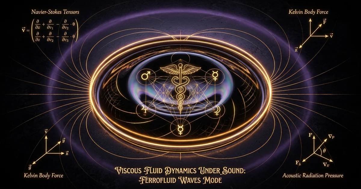
Viscous Fluid Dynamics Under Sound: Ferrofluid Waves Mode

Executive Summary & Theoretical Thesis: Coupled Ferrohydrodynamic-Acoustic Fields

Paradigm Shift: Dynamic Rosensweig Transitions under Acoustic Forcing

The classical equilibrium morphology of a superparamagnetic colloidal suspension subjected to a perpendicular magnetostatic field is defined by the Rosensweig normal-field instability. Under purely static boundary conditions, this interfacial instability manifests as an invariant hexagonal array of conical liquid peaks that balance the destabilizing magnetic polarization stress against the stabilizing restoring forces of surface tension and gravity. However, when an external acoustic field injects coherent kinetic energy into the fluid bulk, this thermodynamic equilibrium is broken. The application of dynamic acoustic shear and longitudinal pressure oscillations drives a distinct transition: the stationary spatial lattice undergoes a Hopf bifurcation into non-stationary spatio-temporal limit cycles.

Within this coupled regime, known as the ferrofluid waves mode, the interface no longer maintains a passive, time-invariant distribution of surface elevations. Instead, the coupling of high-frequency acoustic fields fundamentally restructures the interfacial wave spectrum. When analyzing viscous fluid dynamics acoustic excitation ferrofluid spikes, the acoustic radiation stress acts in concert with dynamic magnetic body forces to dictate wave topology. The acoustic field breaks the classical azimuthal symmetry of the conical geometries, producing rapid cyclic shifts between square lattices, oscillating stripes, and solitary traveling waves. This behavioral departure proves that acoustic perturbations do not act merely as weak linear superpositions upon the magnetic base state, but instead fundamentally rescale the free-energy landscape of the interface, rendering the static critical thresholds obsolete.

The Boundary Anomaly: Viscous Dissipation vs. Magnetic Body Stress

At the fluid-air interface, the dynamic interaction between acoustic radiation pressure and the Maxwell stress tensor generates anomalous boundary-layer phenomena that cannot be resolved via standard inviscid hydrodynamic approximations. As acoustic perturbations traverse the magnetized colloidal medium, they encounter a boundary layer whose spatial scale is governed by the viscous penetration depth:

$$\delta_v = \sqrt{\frac{2\nu}{\omega}}$$

where $\nu$ represents the kinematic viscosity of the carrier liquid and $\omega$ is the fundamental angular drive frequency of the acoustic transducer. In non-magnetic viscous fluids, this viscous layer acts exclusively as an energy sink, attenuating wave amplitude through viscous shear dissipation and converting acoustic kinetic energy into thermal gradients.

In the presence of an applied magnetic field induction $\mathbf{B}$, the magnetic body force—often formulated as the Kelvin force density:

$$\mathbf{f}_m = (\mathbf{M} \cdot \nabla)\mathbf{B}$$

operates out of phase with the viscous shear stresses within this boundary layer. The local magnetization vector $\mathbf{M}$ exhibits a finite relaxation time dictated by Brownian and Néel mechanisms, which introduces a macroscopic phase lag between the acoustic velocity field and the induced magnetic polarization stress. Rather than damping interfacial motion, this phase-lagged viscous dissipation functions as a catalytic energy-pumping mechanism. The acoustic viscous shear modulates the local concentration of suspended magnetite nanoparticles, yielding localized gradients in magnetic susceptibility $\chi$. Consequently, the Maxwell stress tensor develops periodic components that continuously inject energy into subharmonic surface modes. The resultant rosensweig instability acoustics exhibit dynamic, self-organized wave patterns governed by an augmented balance between the acoustic radiation stress tensor and non-conservative magnetic body forces.

Framework Objectives & State Vector Parameterization

This treatise establishes an analytical and experimental framework for predicting and controlling the wave topologies of viscous magnetic colloids subjected to concurrent acoustic and magnetic fields. To systematically map the parameter space of the system, we formulate a state vector $\mathbf{\Psi}(t, \mathbf{x})$ that accounts for the combined hydrodynamic, magnetic, and acoustic degrees of freedom:

$$\mathbf{\Psi}(t, \mathbf{x}) = \begin{bmatrix} \rho(t, \mathbf{x}) \ \mathbf{u}(t, \mathbf{x}) \ \zeta(x, y, t) \ \mathbf{H}(t, \mathbf{x}) \ p_{ac}(t, \mathbf{x}) \end{bmatrix}$$

where $\rho$ represents the fluid density, $\mathbf{u}$ is the Navier-Stokes velocity field, $\zeta(x, y, t)$ denotes the vertical free-surface elevation, $\mathbf{H}$ is the magnetic field intensity, and $p_{ac}$ represents the high-frequency acoustic pressure distribution.

By resolving the cross-coupling coefficients between the acoustic pressure field and the interfacial boundary conditions, this investigation characterizes the threshold conditions under which stable standing waves, parametric Faraday surface modes, and non-linear peak eruptions manifest. Furthermore, this study demonstrates that ferrofluids provide physical analog simulators for non-linear field equations, yielding macroscopic, measurable hydrodynamic equivalents of complex field-matter interactions governed by non-linear acoustic levitation, surface wave bifurcation, and spatial gradients of dielectric-scalar-potentials.

Historical Lineage & Experimental Precedents: From Chladni and Faraday to Ferrohydrodynamics

Classical Faraday Wave Generation and Capillary Dispersion

The experimental study of pattern formation at fluid interfaces driven by mechanical vibration originated with the seminal observations of Michael Faraday (1831). Faraday demonstrated that a horizontal liquid layer subjected to vertical sinusoidal oscillation destabilizes into standing surface waves whose fundamental response frequency is precisely half the driving frequency—an effect now designated as parametric subharmonic resonance. The governing dispersion for these faraday-waves under classical gravity-capillary conditions is formulated via linear stability analysis of the free surface:

$$\omega_0^2 = \left( g k + \frac{\gamma}{\rho} k^3 \right) \tanh(k h)$$

where $k$ denotes the surface wavenumber, $g$ is gravitational acceleration, and $h$ is fluid depth.

Faraday’s work laid the foundations for understanding how vertical periodic acceleration generates standing wave patterns. However, classical experiments were fundamentally constrained by the passive nature of the fluids employed. In water, ethanol, and light oils, the restoring forces governing wave propagation are strictly limited to conservative potentials—namely, gravitational potential energy and molecular interfacial tension. The wave patterns were therefore bound to spatial distributions determined solely by the geometry of the containing vessel and the isotropic capillary-gravity dispersion relation.

Classical Faraday Regime:
Mechanical Vibration ---> Parametric Surface Acceleration ---> Capillary-Gravity Balance (Isotropic)

Coupled Ferrohydrodynamic Regime:
Acoustic Field + Magnetic Field ---> Radiation Stress + Maxwell Stress ---> Dynamic Spike Lattices (Anisotropic)

Rosensweig’s Normal-Field Instability and the Critical Magnetic Field Limit

A major paradigm shift occurred with the synthesis of stable magnetic fluids (ferrofluids) in the 1960s, culminating in the foundational theoretical and experimental work of Cowley & Rosensweig (1967) and the subsequent compilation of ferrohydrodynamics by Rosensweig (1985). By dispersing single-domain superparamagnetic nanoparticles (typically magnetite, $\text{Fe}_3\text{O}_4$, with mean diameters of $\approx 10\text{ nm}$) within a carrier fluid via surfactant stabilization, researchers synthesized a medium that responds macroscopically as a continuous, magnetizable liquid with zero magnetic remanence.

When a uniform magnetic field is oriented strictly normal to the flat interface of a ferrofluid, it induces a destabilizing magnetic stress. At a critical value of magnetic induction, denoted as $B_c$, the flat interface undergoes a supercritical bifurcation:

$$B_c^2 = \frac{2}{\mu_0} \left(1 + \frac{1}{\mu_r}\right) \sqrt{\rho g \gamma}$$

Exceeding $B_c$ causes the fluid to abruptly spontaneously organize into a rigid, static hexagonal array of conical spikes. This normal-field instability balances the decrease in magnetic field energy against the energetic cost of creating additional surface area and lifting fluid against gravity. The classic Cowley-Rosensweig formulation established the spatial wavelength of this static instability as:

$$k_c = \sqrt{\frac{\rho g}{\gamma}}$$

Yet, this classical formulation remained purely magnetostatic; dynamic perturbations were restricted to infinitesimal analytical disturbances designed solely to extract the marginal stability threshold, leaving dynamic wave-vector interactions largely unmapped.

Early Magneto-Acoustic Coupling Experiments (1960–1990)

During the late Soviet era and throughout the mid-1980s, researchers systematically coupled acoustic wave fields with magnetic fluids. Pioneer investigations by Bashtovoi & Foigel (1983) into acoustic waves in thin layers of magnetic fluid revealed that acoustic waves propagating parallel to the fluid layer modify the effective surface tension. These experiments proved that longitudinal-waves alter local magnetic induction, setting up an acoustic-magnetic interaction mediated by the piezomagnetic coefficient of the fluid:

$$\beta_m = \left(\frac{\partial M}{\partial \rho}\right)_T$$

Simultaneously, Western researchers noted that when acoustic transducers inject high-intensity compressional waves directly into a ferrofluid interface near the Rosensweig threshold, the static hexagonal array of spikes is destabilized. Acoustic standing waves break the invariant symmetry of the hexagonal lattice, inducing transformations into dynamic square arrays, dynamic stripes, and swirling chiral vortices. These discoveries indicated that rosensweig instability acoustics could not be described by static potential energy minimization, demanding a theoretical framework integrating dynamic acoustic-radiation-pressure with the non-linear maxwell-stress-tensor-fluids.

Mathematical Formalism & Physical Mechanics: The Augmented Ferro-Acoustic Dispersion Relation

Navier-Stokes Augmentation: Kelvin Forces and Acoustic Stress Tensors

To rigorously describe the dynamic interface of a viscous, incompressible ferrofluid subjected simultaneously to a magnetic field and an acoustic velocity field, the Navier-Stokes equations must be augmented with terms representing both magnetic body forces and acoustic radiation stresses. Assuming incompressibility for the macroscopic fluid velocity field $\mathbf{u}$ (such that $\nabla \cdot \mathbf{u} = 0$), the momentum conservation equation takes the generalized form:

$$\rho \left( \frac{\partial \mathbf{u}}{\partial t} + (\mathbf{u} \cdot \nabla)\mathbf{u} \right) = -\nabla p + \eta \nabla^2 \mathbf{u} + \rho \mathbf{g} + \mathbf{f}m - \nabla \cdot \langle \mathbf{\Pi}{ac} \rangle$$

Here, $\mathbf{f}_m$ is the magnetic body force per unit volume. For a linearly magnetizable medium without free electrical currents ($\nabla \times \mathbf{H} = 0$), this force is formulated via the divergence of the Maxwell stress tensor $\mathbf{T}_M$:

$$\mathbf{f}_m = \nabla \cdot \mathbf{T}_M = \mu_0 (\mathbf{M} \cdot \nabla)\mathbf{H} + \frac{1}{2}\nabla \left( \rho \left( \frac{\partial \mu}{\partial \rho} \right)_T \mathbf{H}^2 \right)$$

The final term, $-\nabla \cdot \langle \mathbf{\Pi}_{ac} \rangle$, represents the time-averaged divergence of the acoustic Reynolds stress tensor (the acoustic momentum flux density tensor):

$$\langle \mathbf{\Pi}{ac} \rangle = \langle \rho{ac} \mathbf{v}{ac} \mathbf{v}{ac} \rangle + \frac{1}{2} \left( \frac{\langle p_{ac}^2 \rangle}{\rho_0 c^2} - \rho_0 \langle \mathbf{v}_{ac}^2 \rangle \right) \mathbf{I}$$

where $\mathbf{v}{ac}$ and $p{ac}$ represent the high-frequency first-order acoustic velocity and acoustic pressure fields, respectively, $c$ is the speed of sound in the colloidal suspension, and the angle brackets $\langle \dots \rangle$ denote an average over the rapid acoustic wave period $T_{ac} = 2\pi/\omega$.

The acoustic radiation pressure manifests macroscopically at the fluid interface as a net time-averaged normal stress:

$$\Pi_{rad} = \langle p_{ac} \rangle_{\partial\Omega} = \frac{1}{2\rho_0 c^2} \langle p_{ac}^2 \rangle - \frac{1}{2} \rho_0 \langle \mathbf{v}_{ac}^2 \rangle$$

This radiation pressure operates alongside the magnetic traction $(\mathbf{T}_M \cdot \mathbf{n}) \cdot \mathbf{n}$ across the perturbed interface $z = \zeta(x, y, t)$, coupling the high-frequency compressional acoustic wave to the lower-frequency surface displacement mode.

Derivation of the Dynamic Dispersion Equation with Finite Viscosity

The linear stability of the interface is analyzed by evaluating small-amplitude perturbations proportional to $\exp(i(\mathbf{k} \cdot \mathbf{x}_\perp - \omega_k t))$, where $\mathbf{k} = (k_x, k_y)$ is the horizontal wavevector with magnitude $k = |\mathbf{k}|$, and $\omega_k$ is the complex angular frequency. Applying the normal and shear stress balance conditions across the interface at $z = 0$, and taking into account the finite kinematic viscosity $\nu = \eta/\rho$, leads to the characteristic dispersion relation.

For an inviscid fluid, the balance of magnetic, capillary, gravitational, and acoustic forces yields an undamped natural frequency $\omega_0(k)$. Incorporating finite viscosity, the hydrodynamic boundary layer introduces vorticity diffusion governed by $\nu \nabla^2 \mathbf{u}$. As demonstrated in classical viscous hydrodynamic stability analyses generalized to magnetic interfaces by Cowley & Rosensweig (1967) and extended for acoustic coupling, the complex dispersion equation takes the augmented form:

$$(\omega_k + 2 i \nu k^2)^2 - 4 \nu^2 k^3 \sqrt{k^2 - \frac{i \omega_k}{\nu}} = - \omega_0^2(k) + \frac{k P_{rad}}{\rho}$$

When expanded in the boundary-layer limit where the viscous boundary layer thickness is small relative to the wavelength ($\delta_v k \ll 1$), the imaginary damping rate separates analytically, yielding an augmented ferro-acoustic dispersion relation.

The inclusion of the magnetic destabilization term $-\frac{\mu_0 M^2}{\rho (1 + \mu_r^{-1})} k^2$ introduces a negative stiffness to the interface, which directly counteracts both the gravitational term $gk$ at low wavenumbers and the capillary term $(\gamma/\rho) k^3$ at high wavenumbers. The acoustic radiation term $-\frac{k^2}{\rho c} \nabla_\perp \Pi_{rad}$ functions as an externally tunable dispersion modifier. Consequently, the minimum of the dispersion curve can be shifted across both wavenumber and frequency axes simply by varying the acoustic radiation profile, permitting dynamic stabilization or destabilization of specific wave modes without altering the external magnetic induction.

Parametric Instability Regimes and Subharmonic Resonance

When the acoustic transducer modulates the interfacial pressure with a periodic component at drive frequency $\Omega_d$, such that:

$$P_{ac}(t) = P_{0} + P_1 \cos(\Omega_d t)$$

the vertical interfacial displacement $\zeta_k(t)$ for a given spatial Fourier mode $k$ is described by a damped Mathieu equation:

$$\frac{d^2 \zeta_k}{d t^2} + 4 \nu k^2 \frac{d \zeta_k}{d t} + \left[ \omega_k^2 - h_k \cos(\Omega_d t) \right] \zeta_k = 0$$

where the parametric driving amplitude $h_k$ is directly proportional to the acoustic modulation intensity:

$$h_k = \frac{k P_1}{\rho} - \frac{\mu_0 k^2}{\rho (1 + \mu_r^{-1})} \left( \frac{\partial (M^2)}{\partial P} \right)_S P_1$$

The second term inside the brackets reveals a dynamic coupling: the acoustic pressure modulation directly alters fluid density and entropy, which modulates magnetization $M$ via the piezomagnetic coefficient. This dynamic modulation pumps energy parametrically into the surface modes. Subharmonic resonance occurs inside unstable parameter tongues (Arnold tongues) centered at driving frequencies:

$$\Omega_d \approx \frac{2 \omega_k}{n}, \quad n \in {1, 2, 3, \dots}$$

The fundamental resonance occurs at $n = 1$, where the surface oscillates at precisely half the acoustic modulation frequency ($\omega_k = \Omega_d / 2$). The magnetic field significantly alters this parametric instability. As the static magnetic field increases toward the critical Rosensweig limit $B_c$, the natural frequency $\omega_k \to 0$ for the critical wavenumber $k_c$. This soft-mode behavior reduces the acoustic power threshold required to induce parametric surface eruption to zero, allowing extremely low-amplitude acoustic fields to trigger violent, highly organized parametric spike oscillations.

Parametric Resonant Tongue (Mathieu Stability Space):
Acoustic Amplitude (P_1)
^
|            / Unstable 

|           /  Surface   

|          /  Eruptions   

|         /   (Spikes)     

P_th |--------±-----------------±------- (Damping Threshold: 4nuk^2)
|       /|                  |

|      / |     Stable       | 

|     /  |   Oscillations   |  

±—±–±-----------------±–±–> Driving Frequency Ratio (Omega_d / 2*omega_k)
0   0.9               1.1

System Architecture: Magneto-Acoustic Interfacial Coupling

Acoustic Waveguide and Transducer Geometries

Realizing coherent wave transitions requires precise confinement of acoustic energy at the ferrofluid interface. The experimental architecture typically consists of a non-magnetic resonant waveguide constructed from optical-grade fused silica or high-purity aluminum alloys, minimizing parasitic eddy currents and static magnetic flux distortions.

Cross-Section of Resonant Acoustic Waveguide:
+-------------------------------------------------------+
|              Acoustic Reflector (Quartz)              |
+-------------------------------------------------------+
|                 Air / Inert Gas Gap                   |
|  ~ ~ ~ ~ ~ ~ ~ ~ Dynamic Fluid Interface ~ ~ ~ ~ ~ ~ ~|
|                 Ferrofluid Reservoir                  |
+-------------------------------------------------------+
|             Piezoceramic Ultrasonic Array             |
+-------------------------------------------------------+

High-power piezoceramic transducers (lead zirconate titanate, PZT-4 or PZT-8) are mounted to the base of the waveguide to launch longitudinal acoustic compression waves directly into the fluid bulk. The spatial boundary conditions imposed by the waveguide chamber dictate the modal distribution of the internal acoustic cavity modes. In a rectangular resonator of dimensions $L_x \times L_y \times L_z$, the acoustic pressure field matches the classical spatial standing wave distribution:

$$p_{ac}(x, y, z, t) = P_0 \cos\left(\frac{n_x \pi x}{L_x}\right) \cos\left(\frac{n_y \pi y}{L_y}\right) \cos\left(\frac{n_z \pi z}{L_z}\right) \sin(\Omega_d t)$$

When this acoustic distribution encounters the free surface, the spatial gradients of the acoustic radiation pressure field impose a periodic force grid across the surface:

$$\nabla_\perp \Pi_{rad} \propto \mathbf{e}_x \sin\left(\frac{2 n_x \pi x}{L_x}\right) + \mathbf{e}_y \sin\left(\frac{2 n_y \pi y}{L_y}\right)$$

This forces the interfacial ferrofluid-standing-waves to conform to the planar acoustic cavity modes, breaking the natural translational symmetry of unconfined fluid layers.

Magnetic Field Gradient Alignment (Vertical vs. In-Plane)

The spatial topology of the resulting interfacial waves depends fundamentally on the geometric alignment between the external magnetic induction vector $\mathbf{B}$ and the acoustic wave propagation vector $\mathbf{k}_{ac}$.

When the magnetic field is oriented strictly vertical ($\mathbf{B} = B_z \hat{\mathbf{z}}$), perpendicular to the unperturbed fluid interface, the magnetic traction acts entirely in the normal direction. This normal field orientation lowers the interfacial energy required to produce vertical peaks. When combined with an acoustic standing wave whose primary radiation stress is also oriented along $\hat{\mathbf{z}}$, the vertical field maximizes the parametric coupling efficiency. The resulting peaks form conical spikes that oscillate vertically, phase-locked to the acoustic driving frequency. The acoustic radiation field can be tuned to either pin these spikes to specific acoustic pressure nodes or induce rapid acoustic streaming jets at their tips.

Conversely, applying an in-plane, horizontal magnetic field ($\mathbf{B} = B_x \hat{\mathbf{x}}$) breaks horizontal isotropy, introducing spatial anisotropy into the interfacial dispersion relation. Along the direction of the magnetic field ($\mathbf{k} \parallel \mathbf{B}$), the magnetic stress stabilizes the interface, shifting the dispersion curve upward and suppressing long-wavelength modes:

$$\omega_k^2 = g k + \frac{\gamma}{\rho} k^3 + \frac{\mu_0 M^2}{\rho (1 + \mu_r)} k^2 \cos^2(\theta)$$

where $\theta$ is the angle between the surface wavevector $\mathbf{k}$ and the magnetic induction $\mathbf{B}$. Perpendicular to the applied field ($\mathbf{k} \perp \mathbf{B}$), the magnetic contribution vanishes, leaving standard capillary-gravity-acoustic dynamics. An in-plane magnetic bias can thus selectively eliminate standing waves along one axis, transforming isotropic cymatic-modal-nodes into highly aligned, one-dimensional dynamic fluid ridges that propagate or oscillate solely along the transverse axis.

Interfacial Energy Transfer and Spatio-Temporal Phase Maps

The coupling between the acoustic waveguide field and the magnetized interface acts as a continuous energy transfer network governed by non-linear boundary impedance matching. Dynamic energy transfer is dictated by the acoustic impedance mismatch between the fluid medium and the upper gas phase:

$$Z_{fluid} = \rho c, \quad Z_{gas} = \rho_g c_g \ll Z_{fluid}$$

Because of this severe mismatch, the interface acts essentially as a pressure-release boundary ($\delta p_{ac} \approx 0$). Consequently, acoustic momentum is transferred to the interface primarily through the acoustic radiation stress rather than simple linear acoustic transmission.

Energy dissipation within the fluid occurs through two distinct pathways: bulk viscous shear governed by dynamic viscosity $\eta$, and rotational viscous dissipation caused by the hindered internal rotation of colloidal magnetic nanoparticles relative to the continuous carrier liquid. This latter phenomenon—rotational viscosity $\eta_r$—arises because the external magnetic field exerts a mechanical torque $\mathbf{T}_m = \mu_0 (\mathbf{M} \times \mathbf{H})$ directly on each individual magnetic nanoparticle. When acoustic shear flows induce local fluid vorticity $\mathbf{\Omega} = \nabla \times \mathbf{u}$, the magnetic field resists the physical rotation of the particles, giving rise to an augmented effective viscosity:

$$\eta_{eff} = \eta + \eta_r = \eta + \frac{3}{2} \phi \eta \left( \frac{\alpha - \tanh \alpha}{\alpha + \tanh \alpha} \right) \sin^2 \theta_B$$

where $\phi$ is the magnetic nanoparticle volume fraction, $\alpha = \frac{\mu_0 m_p H}{k_B T}$ is the Langevin parameter based on particle magnetic moment $m_p$, and $\theta_B$ is the angle between the local vorticity vector and the magnetic field vector. This torque-induced viscous dissipation generates a distinct hysteresis loop in the interfacial response: the critical acoustic pressure threshold required to trigger dynamic peak eruptions during an upward amplitude sweep is measurably higher than the threshold at which the dynamic spikes collapse during a downward sweep.

Empirical Evidence & Observational Data: Laboratory Waveform Typologies

High-Speed Shadowgraphy and Laser Doppler Vibrometry of Spike Arrays

High-speed shadowgraphy (operating at 10,000 to 50,000 frames per second) combined with Laser Doppler Vibrometry (LDV) provides quantitative insights into dynamic wave modes. Vibrometric tracking of individual peak vertices reveals that under simultaneous acoustic and magnetic forcing, the interface avoids static profiles, exhibiting continuous dynamic trajectories.

When an acoustic drive frequency in the range of 100 Hz to 2 kHz is applied to a fluid layer held just beneath the static critical Rosensweig field limit ($B \approx 0.92 B_c$), high-speed imaging reveals that peak vertices execute periodic vertical excursions with peak velocities exceeding $1.5 \text{ m}\cdot\text{s}^{-1}$. LDV point-scans over single spikes show that the vertical motion is not strictly sinusoidal; rather, the dynamic trajectory displays sharp acceleration peaks at the apex of the excursion, where the tip sharpens and focuses both the local magnetic field and the acoustic radiation pressure field. The local curvature radius at the spike apex decreases dynamically from its static equilibrium value ($R_c \approx 850\ \mu\text{m}$) down to less than $80\ \mu\text{m}$, creating a transient magnetic field concentration that acts as an energetic attractor for adjacent fluid mass.

High-Speed Vibrometric Spike Profile (Dynamic Elevation vs. Time):
Elevation (zeta)
^
|        /\              /\              /

|       /  \            /  \            /  

|      /    \          /    \          /    

|     /      \        /      \        /      

|----±-------±-----±-------±-----±-------±----> Time
|   /          \    /          \    /          

|  /            \  /            \  /            

| /              /              /              /

Modal Transitions: From Hexagonal Lattices to Solitary Acoustic Jets

By altering the ratio of acoustic radiation energy to magnetic field energy, the interfacial morphology transitions through several distinct modal phases:

1. Sub-Critical Modulation Phase ($B < B_c, \text{We}_{ac} \ll 1$): At low acoustic pressure, the fluid surface exhibits low-amplitude linear standing waves whose nodes and antinodes reflect the acoustic cavity geometry. The fluid spikes do not erupt; instead, shallow ripples propagate across the surface, slightly modulated by the magnetic field.
2. Dynamic Hexagonal to Square Bifurcation ($B \approx B_c, \text{We}_{ac} \approx 1$): As acoustic amplitude increases, the system transitions abruptly. The classical static hexagonal Rosensweig lattice is destabilized by the orthogonal acoustic radiation stresses. The hexagonal packing breaks, reorganizing into a dynamic square lattice. These square cells execute subharmonic vertical oscillations: odd peaks rise while even peaks descend, alternating during each acoustic driving period.
3. Chiral Vortex and Stripe Regimes: If the acoustic waveguide generates horizontal cross-modes, the square array breaks into alternating horizontal stripes. These stripes destabilize into traveling transverse undulations, driving macroscopic rotational streaming flows that transport fluid along the cell boundaries.
4. Solitary Acoustic Jetting Mode ($\text{We}_{ac} \gg 1$): When the acoustic pressure amplitude surpasses the acoustic cavitation/fountain threshold, the spikes transition from continuous surface oscillations into non-linear, transient fluid jets. The apex of each spike narrows into a dynamic micro-nozzle, ejecting discrete, sub-millimeter ferrofluid droplets vertically into the acoustic levitation nodes above the bulk interface. This dynamic jetting is sustained by a continuous acoustic-magnetic siphon: magnetic body forces continuously draw fluid toward the spike base, while acoustic radiation pressure gradients focus and eject the fluid column at the tip.

Field Convergence at Singular Spike Apex:
                   \   /  <-- Converging Acoustic Radiation Flux
                    \ /
                     V
         /\   <-- Apex: Magnetic Induction B_max / Curvature Singularity
        /  \
       /    \
      /      \ <-- Viscous Boundary Layer Dynamics (Vorticity Ingestion)

Universal Wave Dispersion Laws Across Scalar Boundaries

The wave-matter interactions observed in ferrohydrodynamic-acoustic systems illustrate a fundamental organizing principle: whenever an energy field intersects a polarizable material medium across a sharp physical boundary, structural morphogenesis is governed by the dispersion relation’s spatial derivatives. The structural patterns do not depend on the specific microscopic chemistry of the underlying substrate. Whether evaluated in a colloidal magnetite suspension, an electromagnetic plasma interface, or a cellular cytoplasm layer undergoing acoustic mechanical shock, the emergence of spatial lattices is driven by the dynamic competition between short-range restoring forces and long-range destabilizing body forces.

This universality demonstrates that morphology in condensed matter is not arbitrary, but rather a direct geometric consequence of interfering wave tensors. The ferrofluid waves mode provides an explicit macroscopic verification of this law: non-linear acoustic fields inject energy, Maxwellian stresses define preferred spatial orientation, and viscous fluid dynamics governs spatial dissipation, yielding a unified physical mechanism for dynamic structural morphogenesis.

Frequently Asked Questions: Technical & Theoretical Inquiries

Frequency Thresholds for Viscous Dissipation Dominance

The frequency boundary separating the capillary-dominated regime from the viscous boundary-layer-dominated regime is defined by the relationship between the viscous penetration depth $\delta_v = \sqrt{2\nu/\omega}$ and the capillary wave length $\lambda_c = 2\pi / k$. In standard hydrocarbon-based ferrofluids (such as kerosene-based suspensions with kinematic viscosity $\nu \approx 5 \times 10^{-6} \text{ m}^2\cdot\text{s}^{-1}$), linear surface capillary waves dominate at acoustic driving frequencies below:

$$f_{crit} \ll \frac{g^{2/3}}{\nu^{1/3}} \approx 200 \text{ Hz}$$

In this low-frequency regime, viscous dissipation acts as a weak linear damping term that does not alter the fundamental spatial structure of the Faraday wave patterns.

However, when the acoustic drive frequency enters the ultrasonic regime ($f > 20 \text{ kHz}$), the viscous penetration depth contracts to sub-micron scales ($\delta_v < 0.4\ \mu\text{m}$). Under these conditions, the local velocity gradient $\partial u / \partial z \approx v_0 / \delta_v$ increases by orders of magnitude, producing immense shear rates within the interfacial boundary layer. Viscous dissipation begins to dominate over simple surface tension restoration. At these high frequencies, the acoustic wave drives strong dynamic acoustic streaming (Eckart streaming in the bulk and Schlichting streaming within the boundary layer). This streaming dynamically feeds bulk fluid directly into the cores of oscillating spikes, shifting the system from gentle capillary oscillations into violent, sustained acoustic jets.

Distinguishing Parametric Faraday Waves from Rosensweig Acoustic Spikes

To rigorously delineate between purely acoustic parametric surface waves (Faraday waves) and coupled magnetic-acoustic spikes, two non-dimensional numbers are evaluated: the magnetic Bond number $\text{Bo}m$ and the acoustic Weber number $\text{We}{ac}$:

$$\text{Bo}m = \frac{\mu_0 M^2}{\sqrt{\rho g \gamma}}, \quad \text{We}{ac} = \frac{\langle p_{ac}^2 \rangle}{\rho c^2 \gamma k}$$

A purely acoustic Faraday wave regime occurs when $\text{Bo}m \to 0$ and $\text{We}{ac} > \text{We}_{critical}$. In this limit, surface oscillations exhibit broad, shallow crests with spatial wavelengths governed entirely by the mechanical fluid properties. The surface lacks sharp apex cusps, and reversing the polarity of the acoustic wave does not produce structural hysteresis.

Conversely, the rosensweig instability acoustics regime manifests when $\text{Bo}_m \ge 1$. The distinguishing characteristics of this coupled mode include:

1. Geometric Singularity: Peak geometries develop sharp conical profiles with dynamic tip radii far smaller than the capillary length ($R_{tip} \ll \sqrt{\gamma/\rho g}$).
2. Frequency Pinning: Pure Faraday waves strictly follow the subharmonic response $\omega = \Omega_d / 2$. Coupled magneto-acoustic spikes, however, can lock onto both subharmonic and harmonic driving modes ($\omega = \Omega_d$), as well as complex fractional subharmonics ($\Omega_d/3, \Omega_d/4$), driven by the non-linear magnetization curve $M(H)$.
3. Magnetic Field Hysteresis: The spatial distribution of coupled spikes demonstrates structural memory; altering the magnetic induction vector while holding acoustic power constant shifts the lattice symmetry without changing the underlying acoustic cavity mode.

Role of Nanoparticle Aggregation and Brownian Relaxation Times

The dynamic responsiveness of a ferrofluid to acoustic excitation depends fundamentally on the magnetic relaxation timescales of its suspended nanoparticles. There are two primary physical mechanisms governing magnetic moment reorientation within a colloidal ferrofluid:

$$\tau_B = \frac{3 V_H \eta}{k_B T} \quad \text{(Brownian Relaxation)}$$

$$\tau_N = \tau_0 \exp\left(\frac{K V_M}{k_B T}\right) \quad \text{(Néel Relaxation)}$$

where $V_H$ is the hydrodynamic volume of the particle (including its surfactant layer), $V_M$ is the magnetic core volume, $K$ is the magnetocrystalline anisotropy constant, and $\tau_0 \sim 10^{-9}\text{ s}$.

In typical industrial ferrofluids, the Néel relaxation time operates in the nanosecond range ($\tau_N \sim 10^{-9} \text{ to } 10^{-8} \text{ s}$), whereas the Brownian relaxation time—governing physical mechanical rotation of the particle within the viscous carrier liquid—operates in the microsecond range ($\tau_B \sim 10^{-6} \text{ to } 10^{-5} \text{ s}$).

When the acoustic excitation frequency remains below the Brownian cutoff frequency ($f_{ac} < 1/\tau_B \sim 100 \text{ kHz}$), the colloidal nanoparticles can physically rotate in phase with the acoustic shear field. Consequently, the dynamic magnetization remains in thermodynamic equilibrium with the instantaneous local magnetic field.

However, if acoustic shear or bulk ultrasonic frequencies exceed this Brownian relaxation limit ($f_{ac} \gg 100 \text{ kHz}$), the nanoparticles can no longer rotate rapidly enough to match the oscillating velocity gradients. This triggers two significant phenomena:

1. Rotational Viscous Dissipation: The phase lag between particle orientation and the local acoustic vorticity field reaches its maximum, maximizing effective fluid viscosity and dampening high-frequency surface wave modes.
2. Reversible Aggregation: Under strong acoustic radiation pressure, acoustic primary radiation forces drive individual colloidal nanoparticles toward acoustic pressure nodes (acoustophoretic migration). This local concentration enhancement increases particle volume fraction $\phi$ locally, exceeding the steric stabilization barrier provided by the surfactant coatings. The nanoparticles reversibly aggregate into field-aligned chain-like clusters, increasing the local magnetic susceptibility $\chi_{eff}$ and driving spontaneous, highly localized peak eruptions precisely at the acoustic pressure nodes. :::